Risk & Uncertainty Analysis

Part of Toolkit for the Economic Evaluation of World Bank Transport Projects

(Institute for Transport Studies, University of Leeds, 2003)

One statement that can confidently be made about any transport project is that the costs and benefits are uncertain. An important question is ‘how uncertain’? By analysing the risk and uncertainty which surrounds the project the probability of a poor outcome can be assessed. In addition, it is often possible to identify ways in which the project can be made more robust, and to ensure that the risks that remain are well managed. Risk and uncertainty analysis is therefore a standard component in the project reporting requirements for World Bank projects. Risk and uncertainty analysis also features other in World Bank tools, such as the RED model (see Note Low Volume Rural Roads [Link]).

This note reviews the general principles of risk and uncertainty analysis in transport (Section 1); and outlines the three principal methods which may be used – sensitivity analysis (Section 2), switching values (Section 3) and Monte Carlo simulation (Section 4). Implications for risk management are given in Section 5 and Further Reading is referenced at the end.

1 GENERAL PRINCIPLES OF RISK AND UNCERTAINTY ANALYSIS IN TRANSPORT

At the start, we can differentiate between risk and uncertainty. Risk is the situation where there is a set of possible outcomes from the project, and the probability of each outcome is known (as in Figure 1(a)). Uncertainty is the situation where there is a set of possible outcomes, but the probability of each one is not known (as in Figure 1(b)). In Figure 1(b), only the expected (or mean) outcome is marked - estimating this is often the focal point of project appraisal in practice, however without some understanding of the likelihood of the predicted outcome, it is worth asking: “how much confidence can be placed in the appraisal results”?

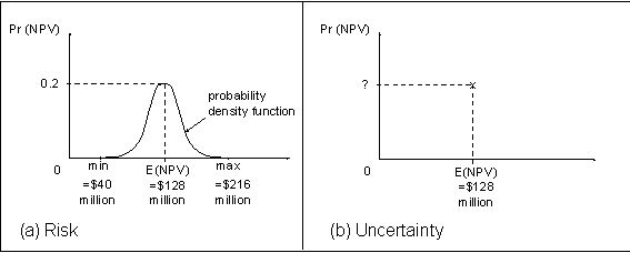
FIGURe 1: RISK VS. UNCERTAINTY

Consider the following example. When we say that the Internal Rate of Return (IRR) of a project is 22% (see Note When and how to use NPV, IRR and Adjusted IRR [Link]), what we usually mean is that the expected outcome (strictly the ‘mean’ IRR) is 22%. Around this is a distribution of possible outcomes. Figure 2 illustrates this, and highlights the 12% Internal Rate of Return which is the usual minimum criterion for acceptability of World Bank projects (see Note When and how to use NPV, IRR and Adjusted IRR [Link]). In this case there is a chance that the IRR may turn out to be less than 12%, but that chance is very small. This type of information is very useful to decision-makers.

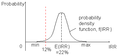
FIGURe 2: A PROBABILITY DISTRIBUTION ON the INTERNAL RATE OF RETURN (IRR)

Once a project is deemed acceptable, the World Bank’s usual decision criterion for projects is then to maximise the expected NPV (see Handbook on Economic Analysis of Investment Operations (World Bank, 1998) [[1]]). It is worth noting that this is not the only possible decision criterion:

- a cautious, or ‘risk averse’ approach, is to maximise the minimum outcome (called the ‘maxi-min’ strategy, for obvious reasons). This would favour projects which are a ‘sure bet’, having only a small downside risk.

- more complex strategies, seeking to balance the risk across a portfolio of investment or to minimise the ‘regrets’ – the consequences of a lower-than expected outcome – are discussed in a range of source books, including Pearce and Nash (1981) [[2]].

In order to make progress with risk analysis in practice, we need to know how the probability distribution in Figure 2 is arrived at? The IRR is determined by the flows of costs and benefits over time, so any riskiness in particular cost or benefit items can be traced through into the IRR. In turn, the risk in each cost or benefit item usually depends on key underlying factors. Box 1 sets out what these factors may be.

Box 1: Sources of risk in transport appraisal

Construction cost risk

It is very common for the costs of major construction projects to be underestimated in appraisal. Underlying reasons for this include:

- engineering risks associated particularly with uncertain ground conditions (geology) and high technology structures, equipment and methods;

- variable input prices, especially energy, labour and imported materials;

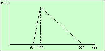
- the complexity of the project management function.

Whether these risks are directly a concern for the purchaser depends on the allocation of risk under the contract. However, even when the risk is fully transferred to the contractor, a premium will usually be charged to bear this risk, so the purchaser continues to face a cost. Figure 2 shows a typical probability distribution for construction cost – most of the risk is downside risk, so the distribution is not symmetrical. So in this case, the expected (mean) value exceeds the most likely value ($120M).

FIGURe: A PROBABILITY DISTRIBUTION ON CONSTRUCTION COST

Operating and maintenance cost risks

These are fuelled by some of the same sources as construction risk, especially rising real labour costs, energy prices and exchange rate risk on imports.

Demand risks – ‘traffic risk’ and ‘revenue risk’

Once a project is complete, the benefits derived from it depend crucially on the forecast user demand being realised. Demand is vulnerable, however, to:

- economic shocks, including fuel price shocks and economic boom or recession;

- changing demographics;

- shifting preferences and growth of competing facilities – eg. roads in competition with rail;

- political intervention;

- random error in the forecasts.

The benefits, in the form of consumers’ surplus, typically decrease as demand decreases. Revenue decreases too, which is an issue for the financial sustainability of projects.

Other risks

Mackie and Preston (1998) [[3]] identified 21 sources of error and bias in transport appraisal. Many of these fall under the general heading of ‘appraisal optimism’, suggesting that downside risks outweigh upside risks in most real situations. HM Treasury (2002), Section 4.11 gives cautionary guidance on this.

2 SENSITIVITY ANALYSIS – ‘WHAT IF’ scenarios

The simplest form of sensitivity analysis involves the creation of ‘what if’ scenarios to reflect the principal risks surrounding the project. Suppose, for example, that a bridge project is believed to be subject to demand risk, because much of the forecast traffic is generated traffic (see Notes Treatment of Induced Traffic [Link] and Demand Forecasting Errors [Link]) which depends on changing patterns of trade and residential location. The analysts responsible for forecasting demand advise that they can only be confident in their forecasts to within +/– 30% of the expected value.

To assess the significance of this risk, the appraiser re-runs the IRR calculation for demand at +30% and –30%, and presents these as ‘what if’ scenarios, in Table 1.

Table 1: SENSITIVITY OF IRR TO DEMAND RISK FOR A BRIDGE

Scenario	Demand in Year 2005, vehicle flow per day	IRR
‘Low’ demand	14,000	13.5%
Expected demand	20,000	16.0%
‘High’ demand	26,000	19.0%

Since the lowest IRR is above the 12% acceptable rate of return, this gives some confidence that the project is robust to the demand risk identified.

3 SWITCHING VALUES

The World Bank’s preferred approach to sensitivity analysis is to calculate switching values. These are the values of the ‘risky’ variables at which the IRR of the project equals the discount rate, and the NPV=0. Table 2 gives an example for the bridge project.

Table 2: SWITCHING VALUES FOR A BRIDGE

Variable	Switching value
Demand (vehicle flow in 2005)	-36%
Construction cost	+44%
Maintenance cost (in 2005)	+70%

Switching values prompt the reader to consider how (un)likely the required switch is, which gives a handle on the robustness of the project to each variable. However, in common with basic ‘what if’ sensitivity analysis, switching values have one great weakness: it becomes complex to understand the risks when several variables are acting simultaneously, rather than one at a time. To explore this, Monte Carlo simulation provides a higher level of analysis.

4 MONte carlo simulation

A leading form of ‘quantitative risk analysis’ Vose (1996) [[4]], Monte Carlo simulation produces a single probability distribution for IRR (or NPV), based on the risk profiles for all the relevant ‘risky’ variables. The method works in the following way:

a) the analyst is required to define a probability distribution for each variable - demand, construction cost, operating cost and so on. This is not as difficult as it sounds (see below).

b) the Monte Carlo procedure then samples randomly from each of the different distributions and calculates the IRR (or NPV), many times over. By taking a very large number of samples from each distribution, the sampling distribution is made to approximate closely the theoretical distribution (Figure 3).

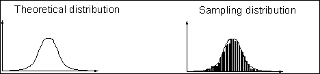
FIGURe 3: THE law of large numbers in application

c) the outcome is a distribution in terms of IRR (or NPV), such as that shown in Figure 1. The more samples are taken, the more stable the distribution becomes.

We said in (a) that Monte Carlo simulation requires information about the probability distributions for each ‘risky’ variable. This is more straightforward than it sounds. For example, based on our understanding of the variable in question we might choose a ‘shape’ for the probability distribution from the set shown in Figure 4.

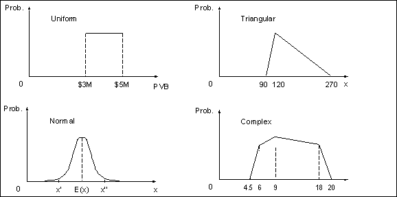
FIGURe 4: Alternative ‘shapes’ for probability distributions

For example, we might adopt a triangular distribution for construction cost. Then by specifying the maximum cost, the minimum cost and the ‘modal’ cost (120 in the Figure), the distribution is fully defined. Alternatively, suppose we judge that demand is normally distributed around the expected flow E(x). We can then fix the distribution by setting the 95% confidence limits on the distribution x’ and x’’.

The simulation itself is carried out by specialised computer software, however, this software is readily available as an add-in to conventional spreadsheet applications and reasonably easy to use. The results will enable the appraiser to report not only the mean value of the project IRR, but also the distribution of the IRR (as in Figure 1) and the cumulative distribution which is useful for representing the probability of meeting the desired rate of return (Figure 5). In this example, there is a 79% probability that the IRR will exceed 12%.

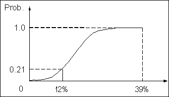
FIGURe 5: cumulative distribution on IRR

Further advice on Monte Carlo simulation is available in the Handbook on Economic Analysis of Investment Operations (World Bank, 1998) [1] and in the many textbooks on the market, such as Vose [4].

5 Risk management

A first step towards effective risk management is risk registration, which includes:

- recognition that a particular set of risks are relevant in planning and implementating the project;

- identification of these risks, and at a very basic level what they are linked to (eg. construction cost of high-technology bridges on a road project; toll road revenues linked to demand growth, in which future income growth and car ownership are key factors; etc.)

Registering risks allows all parties within a project to remain aware of risks, and to monitor development of known risks as a project progresses. The risk register might contain quantitative information about risk – if any is available – and even a description of the type of probability distribution it is believed to follow.

More pro-actively, the project planner can think about prevention, control and transfer of risks. Prevention may be possible by, for example, choosing tried-and-tested solutions in place of riskier innovative ones. Another measure which can play a major role in preventing risk is a comprehensive maintenance programme, which is both designed and implemented to ensure that both level of service delivered by transport assets and the costs of operation remain in line with the project plan (see Note Treatment of Maintenance [Link]. Risk control may be exercised by setting up monitoring systems which can alert project managers to emerging problems. Risk transfer can be used at the contract drafting stage to balance risk and reward for each partner in the contract – including the public sector and private partners [[5]].