Alternatives to the Rule of a Half in Matrix-Based Appraisal

1. BACKGROUND

The ‘rule of a half’ is in widespread use as a measure of the user benefits in transport appraisal. In the UK, it is the measure that is recognised in the official methodology for multi-modal studies (DETR, 2000, Appendix F Section 5) and which is built into the TUBA appraisal software (White, Gordon and Gray, 2001 at this conference).

Rule of a half:

(1)

where GC is the generalised cost of ij travel by mode m;

T is the number of ij trips per period by mode m;

Superscripts ⁰ and ¹ denote the Do-Minimum and Do-Something scenarios respectively; and

CS and GC are at market prices.

However, in three plausible types of situations, the rule of a half is known to break down. These are:

i) large generalised cost changes (for example, as a result of a new estuarial crossing, or a substantial new toll, between i and j on existing mode m);

ii) the introduction of new modes (for example, the introduction of LRT between i and j);

iii) new generators or attractors of trips (for example, due to a major development at a particular location).

All three are of increasing relevance at the present time, as transport policy moves towards new-mode solutions, road infrastructure charging and integrated transport-land use strategies in a number of countries.

This paper puts forward an alternative benefit measure - called ‘numerical integration’ - which can be used selectively as an alternative to the rule of a half. It is valid whatever type of demand model is being used, and extends rather than overturns the logic of the rule of a half. Numerical integration is shown to improve the accuracy of benefit estimation in the first two of the problematic cases above, and the analysis offers some insights into how to deal with case (iii) land use change (Sections 2,3 and 4).

Issues which arise when implementing numerical integration are addressed within each Section, and the specific question of implementation in software is considered. A spin-off from the development of numerical integration is a mathematical proof which extends the generality of the rule of a half (see Section 5). Finally, conclusions are drawn for future appraisal practice (Section 6).

The paper reports on work commissioned by DTLR (then DETR) from the Institute for Transport Studies, to examine the problem and recommend practical solutions. It is expected that the official advice on these matters will be prepared shortly. Exposure of this paper to comment and discussion will help, it is hoped, to inform that advice and give professionals an opportunity to input.

2. LARGE COST CHANGES

2.1 Reasons for the breakdown of the rule of a half

In order to explain the breakdown of the rule of a half (RoH) when cost changes are large, we begin by setting out the standard justification for the use of the RoH.

The first and simplest version of the argument for the RoH is based on the assumption of a single generalised cost change (eg. a reduction in travel time from i to j by road). Supply conditions are assumed to change in one market only and no demand curves in any market shift. There is only one product to consider in the appraisal, with no close competition and no complementarity with other products. A good example of this situation in the real world would be a road improvement project between two rural communities, where the best alternative route is so long that no-one would consider using it.

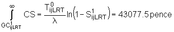
In essence, the rule of a half (RoH) is a linear approximation to the Marshallian consumer surplus measure of benefits¹ (DCS):

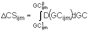(2)

As (3)

where GC is the generalised cost of ij travel by mode m;

D is the demand for ijm trips per period (a function of GC_ijm);

Superscripts ⁰ and ¹ denote the Do-Minimum and Do-Something scenarios respectively, as before; and

CS and GC are both at market prices.

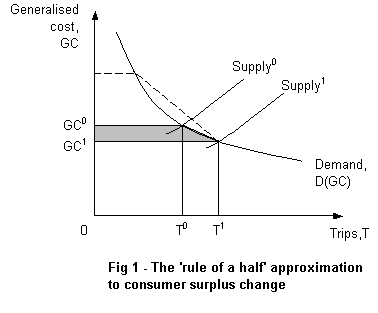
This is illustrated in Figure 1 for a strategy which shifts supply conditions.

The RoH is a good approximation when price changes are small. However, when price change is large (eg. shown by the dotted line), the linear approximation becomes inaccurate. How inaccurate becomes clear in Section 2.3 when a numerical example is considered.

The second version of the justification for the RoH is more complex. In situations where demand curves can shift - for example, decongestion on a road link following the introduction of a parallel LRT - the rule of a half can still be applied to estimate the user benefits, subject to certain conditions holding. The principal conditions are that the change in costs remains small, and that there is symmetry of substitution between the services involved (Jones, 1977; Glaister, 1981). When the generalised cost change is large, this logic also breaks down.

As part of the background for our work, Hyman (2001) has provided a mathematical proof of the validity of the RoH for the joint consumption of related products - see Section 5. However, the conclusion remains that the larger cost change, the less reliable (potentially) the RoH becomes: an alternative benefit measure is needed.

2.2 Numerical integration

‘Numerical integration’ involves defining a set of trapeziums which together approximate the change in consumer surplus. The Do-Something and Do-Minimum points used for the RoH calculation (T⁰,P⁰) and (T¹,P¹) are retained, and supplemented by additional points. Figure 2 illustrates how the method works - the shaded areas indicate the (estimated) user benefits.

Each trapezium, and in fact each triangle, can be calculated using the rule of a half, so the process is simple once the additional points have been defined.

For numerical integration with three additional points (T^a_ijm,GC^a_ijm), (T^b_ijm,GC^b_ijm) and (T^c_ijm,GC^c_ijm). Let these GC levels be:

GC^a_ijm = 0.25*(GC⁰_ijm-GC¹_ijm) + GC¹_ijm (4)

GC^b_ijm = 0.5*(GC⁰_ijm-GC¹_ijm) + GC¹_ijm

GC^c_ijm = 0.75*(GC⁰_ijm-GC¹_ijm) + GC¹_ijm

Given these three levels of generalised cost between i and j by mode m, the forecasting model must be run to determine the corresponding T^a, T^b and T^c.

The numerical integration function (NI) is then:

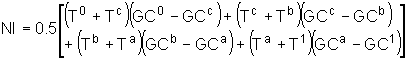(5)

with the ijm subscripts omitted for clarity.

Three advantages of numerical integration that are immediately apparent are:

- it appears to be general - no specific analytical forms of the demand function need to be assumed, hence NI can be used with logit demand models, negative exponential and any other functional forms;

- related to this, knowledge of the demand function is not required in order to estimate the user benefits - this could be a big advantage for more complex demand models, where there may not even be a single explicit demand function in each market;

- numerical integration is highly consistent with the standard treatment of existing modes, as it requires only explicit trip and cost matrices for the mode of interest.

2.3 Worked example: an estuary crossing

In this section, we use a worked example to explore how numerical integration can be applied in matrix-based appraisal. The example uses a very small matrix, but the method can be applied to matrices of any size - we return to the practical issues raised in large matrices at the end.

Suppose that there are two zones in an urban network, separated physically by a river or estuary. Let these be zones 1&2. The shortest route linking 1&2 crosses the river between two neighbouring zones, 3&4. The figure below (Fig 3) illustrates the situation. A project is proposed to link the first two zones directly, across the estuary. To appraise this project, an estimate of the potential user benefits is needed.

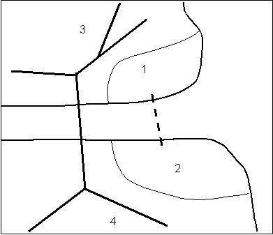
Figure 3: Estuarial crosssing in a network

User benefits may arise across a range of modes, including private car, bus, rail (if the new crossing carries a railway), cycling and walking. Benefits relating to all these modes are relevant in multi-modal appraisal. For simplicity however, we will confine the analysis to just one of these - private car - and to one trip purpose - non-working- and one time of day - peak.

In order to make the benefit calculations we require some information about travel conditions for this demand segment between zones 1&2, so we assume the following (Table 1). It was also supposed that the crossing is not tolled.

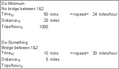
Table 1: Estuary crossing example: short scenario descriptions

Values of time and vehicle operating costs were taken from the Transport Economics Note (DETR, 2001), yielding the following generalised costs (GC₁₂) at 1998 prices and values, assuming that all trips used the lowest generalised cost route.

	Do-Minimum	Do-Something
Time	549.9	110.0
VOC	315.7	72.6
TOTAL	865.7	182.6

Table 2: Estuary crossing: generalised costs, pence per trip

To simulate the transport modelling stage, a base number of trips from zone 1 to 2 was assumed: 1000 per period in the Do-Minimum scenario. A demand function was taken from the SATURN modelling procedures for elastic assignment (T=T⁰exp(-b(GC-GC⁰)) using a demand sensitivity coefficient b=0.0037. A number of further simplifying assumptions were made:

- travel between zones 3 and 4 will continue to be quickest and cheapest via the old bridge across the estuary, not through zones 1&2, and will be unaffected by the project to any significant degree;

- intra-zonal travel will not be affected by the project;

- travel from zones 1 to 4 and 2 to 3 (and vice versa) will be made easier by the project, but given the overall distance involved generalised costs will not fall by a large amount.

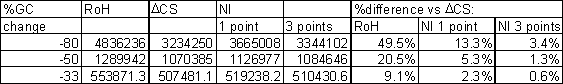
The projected demand response to various large cost reductions including the extremely large cost reduction shown in Table 1, was as shown in Table 3.

% cost D	GC⁰	GC¹	T⁰	T¹
-80	865.7	173.1	1000	6487.3
-50	865.7	432.8	1000	3217.7
-33	865.7	580.0	1000	2162.6

Table 3a: Estuary crossing: demand response to large cost reductions (zone 1 to zone 2)

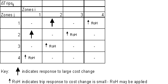
Table 3b: Estuary crossing: demand response across the network

Therefore to estimate the user benefits of the project for this demand segment (car, non-working, peak hour), the rule of a half can be used to estimate the benefits for most cells in the matrix. However, for (1,2) and (2,1) we have the opportunity to test alternative benefit measures. These are:

- the rule of a half - ie a conventional appraisal;

- the integral consumer surplus - the theoretically correct benefit measure, not usually calculated because of the practical difficulties; and

-
numerical integration- with one or three additional points.

Table 4: Estuary crossing: alternatives measures of user benefits

Table 4 gives the benefit estimation results and the error due to the use of firstly the rule of a half and secondly the new benefit measure, numerical integration. These results suggest that the RoH is seriously inaccurate (>10%) for cost changes of >33%. This finding is supported by wider experimentation, in which not only the size of the cost change but also the elasticity coefficient on the demand function were allowed to vary.

It should be noted also that we found before that large changes in trips are no more or less problematic than large changes in costs, in terms of the inaccuracy they cause in the RoH. Therefore the suggested rule for use of NI relate to large trip changes as well as large cost changes. These rules and other practical implementation issues are discussed in the following Section.

2.4 Implementation issues

The key issues identifed during our work were:

1. When is it advisable to use numerical integration in place of the RoH?

2. How many additional (T,GC) points are needed?

3. What is involved - in practical terms - in obtaining Trip estimates for these points?

On the first and second issues, the following rules for intervention are proposed. These are based on experimentation, and except in the case of extremely curved demand functions (for example, an exact reverse L shaped curve), they should usually be adequate to report the benefits accurately to within +/-10% (Nellthorp and Mackie, 2001).

Magnitude of cost and trip changes	User benefit estimator
If % change in P_ijm<33% AND % change in T_ijm<33% then	RoH
If % change in P_ijm33% OR % change in T_ijm33% then	Numerical integration with 1-3 additional points

Table 5: Suggested rules for implementation

In choosing the number of additional (T,GC) points, we have found that NI with 1 additional point brings acceptable accuracy (+/-10%) for cost changes up to roughly 70%. For larger cost changes, NI with 3 additional points brings improved accuracy, at a cost in terms of calculations necessary. Table 4 illustrates this using the numerical example.

The third issue warrants some discussion too. Additional data to implement NI would be generated by re-running the forecasting model for different levels of perceived (generalised) cost for the ijm option concerned. In doing this, care should be taken to ensure that perceived costs are measured in the standard unit of account for TUBA inputs, which is factor cost for work travel and market prices for non-work travel.

When specifying the additional model runs, it is suggested that the definition of the project should be used to help identify the intermediate levels of generalised cost. Thus in the estuary crossing example, the GC level halfway between GC⁰ and GC¹ was obtained by setting ij journey time and distance approximately halfway between their original two levels. It is not necessary for the intermediate points to be exactly evenly spaced - indeed it is recognised that given the need for model equilibrium it may be impossible to fix absolutely exactly on the target value. Numerical integration can give improvements in accuracy without such rigid precision in these GC levels.

These rules could be refined in future in the light of practice using this method with real multi-modal study data. There is obvious scope for adjustment of the number of additional data points, and/or the threshold values of ‘% change in trips’ and ‘% change in cost’, and/or the use of a single threshold.

2.5 Disaggregation into components

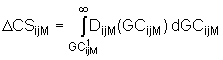
This is fairly straightforward, although as with the conventional RoH calculations, taxes and unperceived costs complicate matters slightly. The NI_ijm calculations for each component are:

user charges: 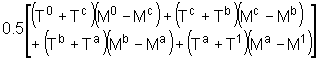(6)

fuel VOCs:

non-fuel VOCs:

travel time:

The components of user benefit to enter into the TEE table are then:

for work trips:

user charges: (7)

fuel VOCs:

non-fuel VOCs:

travel time:

for non-work trips:

user charges:

fuel VOCs:

non-fuel VOCs:

travel time:

3. NEW MODES

3.1 Reasons for the breakdown of the RoH

For a new mode between i and j, the trips and costs in the do-something scenario are known from the transport model outputs: (T¹_ijM, GC¹_ijM). In the do-minimum scenario, trips on the new mode T⁰_ijM=0. However, the do-minimum generalised cost for this mode between i and j is undefined (or infinite), because the mode does not exist for that ij pair in that scenario. This implies that the RoH is also undefined (or infinite).

Consumer surplus for a new mode is given by the integral above the Do-Something generalised cost - see Figure 4. This can be a definite integral if the demand curve intersects the GC axis or an improper integral if the demand curve is asymptotic to it. In general, user benefit of a new option is defined as:

(8)

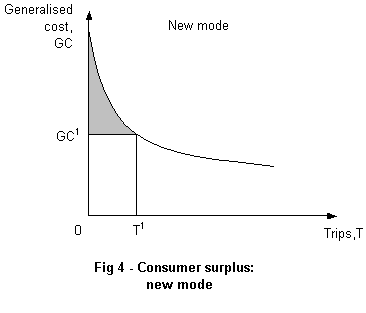
The question is: how best to estimate this consumer surplus?

3.2 Solutions proposed previously

The first and in some ways most appealing answer is: calculate the integral directly. There are some significant obstacles to this, however:

- the demand function in the transport model may not be expressed in such a way that it can readily be integrated: hierarchical choices and discontinuous functions are key sources of difficulty;

- the values and coefficients in the transport model must be identical with those used in appraisal, to ensure consistency across modes and cells in the appraisal;

- the functions of modelling and evaluation are often separated physically and in time, which places a great deal of emphasis on the data transfer between them: to pass non-standard information such as the specification of potentially complex demand functions between the two could be an invitation for errors and misinterpretations.

In view of these difficulties with the integral consumer surplus, the Common Appraisal Framework (MVA, OFTPA and ITS, 1994, Appendix D) proposed a number of pragmatic alternatives. These included:

a) the rough estimation of demand curves for the new mode by fixing a cost intercept on the GC axis and then connecting this to the known point (T¹_ijM, GC¹_ijM) by a straight line;

b) assuming that the demand function could be represented by a binary logit function and using professional judgement to estimate the scaling factor l;

c) using the rule of a half further up the choice hierarchy, to avoid having to calculate CS for new modes at all.

Each of these has some more and some less apparent weaknesses, many of which were recognised in the Common Appraisal Framework itself. A full critical discussion is given in our report (Nellthorp and Mackie, 2001). DTLR was still looking, therefore, for a more robust, standardised approach to estimating the consumer surplus for new modes. Ideally, the approach should be implementable in software - for example as an extension of TUBA.

3.3 Numerical integration for new modes

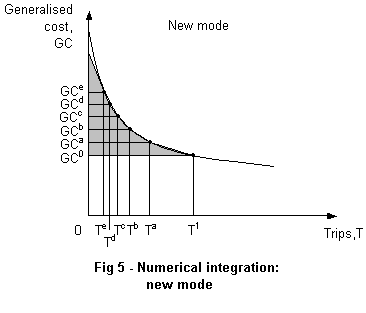
Numerical integration provides a way of obtaining most of the accuracy of the integral CS without requiring knowledge of the demand function.

To obtain an estimate of user benefits by numerical integration in the case of a new mode M, it is necessary to determine GC_ij_M, and the corresponding trip matrices T_ij_M, for a number of hypothetical levels of perceived generalised cost. Let us call these hypothetical scenarios a,b,c and so on. The additional input data required is:

(T^a_ijM,GC^a_ijM) (9)

(T^b_ijM,GC^b_ijM)

(T^c_ijM,GC^c_ijM)

(T^d_ijM,GC^d_ijM)

(T^e_ijM,GC^e_ijM)

for all those i-j pairs between which the new mode M is introduced. Equal spacing of data points in terms of cost is recommended between GC^e and GC¹. Hence GC^d_ijM = 0.8*(GC^e_ijM - GC¹_ijM) + GC¹_ijM and so on.

This data would be generated by re-running the forecasting model for different levels of perceived generalised cost for the new mode. In doing this, care should be taken to ensure that perceived costs are measured in the standard unit of account for TUBA inputs, which is factor cost for work travel and market prices for non-work travel. TUBA itself makes the correction to market prices for work travel (Mott MacDonald, 2001).

The numerical integration function is:

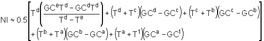
(10)

Incorporating this function directly in matrix-based appraisal would involve programming the software to accept multiple scenarios a to e simultaneously as input data. If this were found to be too difficult, for example if the TUBA data structure is now rigidly fixed in terms of the number of scenarios that can be manipulated at once, an alternative would be to implement the method as a series of TUBA runs with pairs of scenarios input as do-minimum and do-something. One of these runs would serve to calculate the upper triangle, the remainder would calculate the trapeziums. The results, calculated using the RoH, would be summed to obtain the same result as equation (10).

3.4 Worked example: a new LRT

Numerical integration has been tested using a hypothetical new LRT route from a suburb i to the city centre zone j. For simplicity, we consider only individuals for whom car is available and we assume that the existing bus option is so infrequent and of such poor quality that it is not a realistic alternative: car and LRT are therefore the only choices.

In general, generalised cost is the sum of: Money cost (fares and VOCs); In vehicle time; Walk time (access and egress); Wait time; Modal constant. Demand was modelled very crudely using a binary logit model taken from the Manchester Metrolink Monitoring Study (Oscar Faber, 1996, Volume 2 Tables C5/6), whose scaling parameter is equivalent to -0.042 utils per minute.

Assumptions were made about the characteristics of the alternatives as follows (Table 6).

GC_ijm components	Mode		Units
	Car	LRT
Money cost (fares & VOCs, parking charges)	200	80	pence per one-way trip
In-vehicle time	15	20	mins per one-way trip
Walk time (access and egress)	5	10	mins per one-way trip
Wait time	0	7.5	mins per one-way trip
Modal constant	-	-13.9	pence per one-way trip

Table 6: LRT example - characteristics of car and LRT

This model and assumptions implied the demand relationship for LRT shown in Figure 6. The prediction in the do-something scenario is for LRT to take a 26.8% mode share.

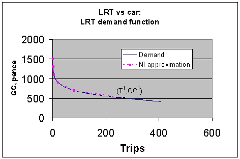
Figure 6: LRT Example: logit demand function and NI approximation

It can be shown that the integral consumer surplus calculation for LRT is:

(11)

where l is the scaling factor in utils per pence = -0.0072;

S¹_LRT is the market share taken by LRT in the do-something.

The points for numerical integration (NI) are as shown in Table 7. Applying the NI formula above gives NI = 47874.6 pence.

	T	GC
e	0.25	1509
d	1	1308
c	5	1107
b	19	905
a	78	704
1	268	503

Table 7: LRT example - points for numerical integration

Thus NI overstates the integral CS by 11.1%, when it is applied with 5 additional points. An alternative approach might be to apply NI with just 3 points (e, c and a) instead of 5. This overstates the true CS by 22.1%.

It is worth noting that in response to comments on the study report, the leftmost point, (T^e, GC^e) has been defined in terms of GC rather than Trips. This should ease the job of implementation, because it is easier (more direct) to input a particular level of GC_LRT into the model than to aim for a particular number of trips, the latter possibly requiring a process trial and error. A tentative assumptions broadly consistent with the analysis do far is that:

(12)

and .

Another suggestion is that this number may depend on the number of additional points.

For comparison, if a rough estimate is made using a straight line through the known point and just one other point on the demand curve - ie. a simple RoH calculation - the scope for inaccuracy is much greater. The % errors are +91.1% if point c is used amd +151.6% if point d is used.

3.5 Implementation issues

The principal implementation issues are:

1. How to define the leftmost point?

2. How many additional (T,GC) points are needed?

We have already noted that the leftmost point could be found by entering supply conditions such that GC_M=3*GC¹_M into the demand model. If there is a demand/supply response which causes equilibrium GC to diverge significantly from the input value (eg. congestion on the new mode), then some adjustment may be needed, although on the whole new modes are probably less likely to suffer from congestion than others.

The number of additional points required has been explored using several numerical examples and typical results suggest that at least 3 points would be needed to reduce the error from 100% to 20%. The addition of further points does not appear to improve the accuracy that much further (not below 10%). In absolute terms, most of the error arises in the lower portion of the demand function: this is, we believe, a consequence of the way the points are specified at equal GC intervals. It may be desirable to refine the advice on this - although whether this is necessary depends partly on the acceptability of a 10-20% error (bearing in mind that the error when new modes are evaluated using other approximate methods is likely to be much greater).

4 NEW GENERATORS AND ATTRACTORS OF TRIPS

The main focus of interest in transport appraisal is usually the benefit due to the Transport strategy (ie. the change in welfare between the Transport Do-Something scenario and the Transport Do-Minimum). However, other policy issues may arise.

There may also be a Land Use strategy. In England, under the new ‘integrated’ regional structure, the Regional Planning Guidance (RPG) incorporates the Regional Transport Strategy (RTS) as well as a regional development and land-use planning policy. It is quite possible, therefore, that policy-makers will wish to see an evaluation of the transport strategy and land use strategy together, as well as the more traditional evaluation of transport strategy alone. Such an evaluation would need to address the (dis)benefits associated with new generators and attractors of trips: physically, these could take the form of new business parks or new towns (such as the proposed ‘Alconbury’ new town in the Cambridge-Huntingdon corridor). In modelling terms, they represent ijm cells in the trip matrix where no trips - or few trips - were made in the Do-Minimum. There is an analogy here to new modes and large trip changes, which we can make use of in thinking about new generators and attractors.

Hyman (2001) supports the conclusions of Jones (1977) and Glaister (1981) that when there is a shift in the partial demand curve for a product - for example ij travel by rail - the RoH can be used to estimate the change in user benefits, provided the income effects are zero. Let us consider what this means in four different appraisal situations.

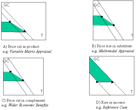
Figure 7: Evaluation using partial demand functions - market interactions

In cases (A), (B) and (C), prices of products change but incomes are assumed to be fixed and the RoH gives the correct change in CS (shaded). However, in case (D) where incomes rise but prices remain fixed, the change in CS is not given by the RoH. In diagram A the shaded area shows the change in consumer surplus for product 1 when there is a reduction in its price and the same time a change in price of a related product. In diagram B the related product 2 is assumed to be a substitute, whose price has risen and the shaded area shows the loss in consumer surplus associated with product 2. In diagram C the related product 2 is assumed to be a complement, whose price has fallen and the shaded area shows the increase in consumer surplus associated with product 2. In diagram D there are no related products and the shaded area shows the increase in consumer surplus associated with product 1 when there is a rise in income.

Now, suppose housing and transport are complementary goods: then by the above reasoning it is appropriate to evaluate price changes for both using the RoH (or NI where necessary). There is no need to hold land use constant when estimating the transport benefits in a Land-Use/Transport Interaction model: they can both be allowed to vary and the RoH will serve to attribute the benefits by ‘source’ between transport and housing, just as it will between modes of transport. If correct, this suggests an amendment may be needed to the advice in GOMMMS (DETR 2000, Volume 2, pB11, Paragraph 2.44).

Going somewhat further, we hypothesise that:

Total benefit = RoH(Transport) + RoH(Land & property) + RoH(Labour)

(13)

RoH(Transport) would be provided by TUBA; the other two would be the subject of separate economic analysis and would be brought together to inform the ‘Wider economic impacts’ line in the New Approach to Appraisal (NATA). This makes an interesting comparison with Martinez and Araya (2000, Fig 1), who conclude that transport sector benefits and land use benefits may not be strictly additive in the presence of transport externalities such as noise nuisance. The full report (Nellthorp and Mackie, 2001) gives some further discussion on this topic.

5. GENERALISATION OF THE RULE OF A HALF

Hyman (2001) gives a mathematical proof of the validity of the RoH in the case of joint consumption of related products, such as the multi-modal appraisal context. There are two related strands of logic.

The first assumes that the willingness to pay for any basket of products can be expressed as a C² (twice continuously differentiable) function of the quantities of each product and proceeds to establish sufficient conditions for the exact application of the rule of a half in the case of multiple related products.

The second uses the multivarite Taylor series expansion of f(), a C² scalar function:

(14)

to demonstrate that:

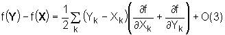(15)

Note that the 1^st order terms are identical to the rule of a half, the second order terms are zero and the third order terms are a possible source of error

Hence in the demand shift/multiple price change case, the RoH gives an approximation that is accurate to second order. The rule can be applied either indirectly to general twice differentiable multi-product WTP functions of quantities or directly to twice differentiable multi-product consumer surplus functions of prices.

When dealing with large price changes or new products the accuracy of the RoH may be insufficient. Provided that we are still dealing with twice differentiable functions, numerical integration may be used to provide the required accuracy.

These results are significant because they verify that the benefit measures embedded in TUBA are appropriate to estimate benefits on inter-related modes, subject to extension to include NI. In particular, they demonstrate that the position taken in GOMMMS (DETR, 2000, Appendix F Para 4.18) is a rather cautious one: it is important to ask why is there is believed to a be a problem with non-uniqueness of attribution of benefits to mode? The results also provide the basis for the novel discussion of the land-use change issue in Section 4.

6. CONCLUSIONS

Alternatives to the rule of a half are needed if we are to have truly general appraisal methods. However, this paper has argued that substantial progress can be made by extending the logic of the rule of half and using the technique of ‘numerical integration’ in selected cases where the RoH breaks down.

Numerical integration appears to be applicable to the estimation of consumer surplus for both existing and new modes, and represents a natural generalisation of the RoH. By applying the RoH in a series of incremental stages a simple, unified and accurate treatment is both possible and practicable.

Numerical integration appears to offer distinct advantages over the alternatives considered. It appears to be general, so that no specific analytical forms of demand function need to be assumed. It is highly consistent with the standard treatment of existing modes, as it requires only explicit trip and cost matrices for the mode of interest, and the accuracy of numerical integration is controllable by varying the number of points.

For large cost changes (>33%) in matrix-based appraisal, we recommend that numerical integration be used with 1-3 additional points. It appears that with 1 point the NI error is about 1/4 that of the RoH, whilst with 3 points it is 1/16 that of the RoH.

For new modes, we recommend that numerical integration be used with 3-5 additional points. This should be sufficient to obtain results accurate to +/-10-20%, a substantial improvement over the other techniques tested.

We recommend that with regard to new generators and attractors, the RoH and NI (as above) be applied as usual, with the land use strategy in place in the do-something if it forms part of an integrated regional strategy. Whatever the land use benefits are, it appears that the transport benefits can be estimated separately using TUBA/NI methods. Similarly, even when the price of the own mode affects the demand on another mode, it is legitimate to add the benefits of one mode to another.

Some refinement of the rules for application may be desirable in the light of experience. Nevertheless, application of these methods should help to ensure that we do not overestimate the benefits of new modes, including LRTs, and conversely that we do not overestimate the disbenefits from large cost increases - eg. due to road user charging - in the future.

NOTE

1. The Marshallian consumer surplus measure is itself a second choice after the ‘ideal’ measure of benefits, which is the compensating variation (CV) (see Jones 1977, Chapter 9; or Glaister 1981, Chapters 2&4). However, provided that the income effects of small changes in the transport system are zero, the consumer surplus can be used to represent CV without introducing any inaccuracy.

REFERENCES

Department of the Environment, Transport and the Regions (DETR) (2000), Guidance on the Methodology for Multi-Modal Studies, DETR, London.

Department of the Environment, Transport and the Regions (DETR) (2001), Transport Economics Note, DETR, London.

Hotelling H (1938), The general welfare in relation to problems of taxation and to railway utility rates, Econometrica 6(3), p242-269.

Hyman (2001), The Applicability of the Rule of a Half to the Consumer Surplus of a Set of Related Products, ITEA Division, DTLR.

Jones IS (1977), Urban Transport Appraisal, Macmillan, London.

Martinez FJ and Araya CA (2000), Transport and land-use benefits under location externalities, Environment and Planning A 32(9), p1611-1624.

Mott MacDonald (2001), TUBA User Manual (Version 1.2), Mott MacDonald, Winchester.

MVA, Oscar Faber TPA and ITS Leeds (1994), Common Appraisal Framework for Urban Transport Projects. Final Report. Department of Transport and Birmingham City Council.

Nellthorp J and Mackie,PJ (2001), Alternatives to the Rule of a Half in Matrix Based Appraisal. Final Report prepared for the Department of the Environment, Transport and the Regions, with contributions by G Hyman and JJ Bates. Institute for Transport Studies, University of Leeds.

Oscar Faber (1996), Metrolink Monitoring Study, Volume Two: Demand Modelling Pre and Post Implementation, Independent Report for the Department of Transport and Greater Manchester PTE, GMPTE, Manchester.

Reaume (1974), Cost-benefit techniques and consumer surplus: a clarificatory analysis, Public Finance 29(2).

Sugden, R. and Williams, A. (1978), The Principles of Practical Cost-Benefit Analysis, Oxford University Press.

White C, Gordon A and Gray P (2001), Economic Appraisal of Multi-Modal Transport Investments: the Development of TUBA. Proceedings of the European Transport Conference.

AUTHORS’ ACKNOWLEDGEMENTS

The authors have benefitted from comments and suggestions by John Bates. They would also like to thank Peter Mackie for his contributions and Robert Sudgen and Dave Milne for helpful discussions. John Nellthorp also acknowledges DTLR’s funding of this work. The conclusions are, however, the authors’ own.

ANNEx 1

Alternatives to the Rule of a Half in Matrix-Based Appraisal