Distribution of Benefits and Impacts on Poor People

(I.T. Transport Ltd, 2003)

Part of Toolkit for the Economic Evaluation of World Bank Transport Projects

(Institute for Transport Studies, University of Leeds, 2003)

Over 1.2 billion people in the world exist on less than the lower poverty threshold of US$1 per day. Therefore, in recent years poverty reduction has become the overarching development objective of developing country governments and international agencies like the World Bank. As the transport sector consumes a considerable part of the overall budget for infrastructure investments in developing countries, there is a need to understand how these investments help with poverty reduction. At the project level the need to demonstrate the contribution of individual projects to poverty reduction becomes inescapable. Given that ethnic, gender and racial inequality are dimensions of as well as causes of poverty (World Bank, 2001), it is also necessary to assess the distributional effects of an investment, or a change in policy, on these groups.

The identification of transport initiatives on poverty and distribution is, however, a complex matter. Primarily this is due to the nature of the interactions between transport and wages, profits, prices and land values let alone gender or racial inequalities. Such interactions are dependent on many factors including the competitiveness of different industries concerned, economic advantages that one region may hold over another, as well as institutional and cultural factors, particularly where gender inequalities are concerned. Techniques for assessing some of these interactions are available (see Note Projects with Significant Expected Re-structuring Effects [Link]. Such techniques, however, are not well developed and consequently will be beyond the resources of most appraisals. Most appraisals will therefore require distributional analysis to be based on the incidence of benefits accruing to travellers and vehicle operators. Whilst not exact such an assessment will at the very least be indicative.

A further issue that has to be considered is the issue of project selection. Without doubt some projects will be more beneficial for the poor than other projects, and some projects will have higher Internal Rates of Return (IRRs) than other projects. The difficulties arise when projects with the highest IRRs have the lowest poverty impacts and vice versa. To this end cost effectiveness analysis is often used as a project screening or sifting tool early in the planning process to ensure that only projects that meet the stated objectives (e.g. those with positive distributional and poverty impacts) are considered (see Note Where to Use Cost Effectiveness Techniques Rather Than Cost Benefit Analysis [Link]).

This note deals with the extent to which, and the means by which, project level distributional analysis of benefits can be undertaken and how poverty impact indicators can be developed[*]. Section 1 sets out the issues associated with using traditional cost benefit analysis for the appraisal of pro-poor projects. Section 2 discusses the techniques and analysis available to consider the distributional consequences of a transport change, whilst Section 3 sets out a number of indicators that can be used for measuring poverty impacts. A summary of the key recommendations is made in Section 4.

1 Economic Efficiency CRITERIA and impacts on poor people

Cost Benefit Analysis (CBA) involves measurement in monetary units of changes in social welfare. As discussed in the Framework [Link] welfare is measured using the surplus criteria – consumer surplus and producer surplus – plus changes in external impacts (e.g. environmental) and government impacts (e.g. tax revenue). Consumer surplus is the difference between the maximum willingness to pay and the market price. While for a tradable commodity market transactions determine willingness to pay, willingness to pay for a non-tradable commodity is determined using preference revelation methods (e.g. valuing travel time savings using stated or revealed preference). The use of willingness to pay means that income can influence the absolute level of benefit as those on higher incomes are often willing to pay more for a unit of benefit than someone on a lower income (see also the Note Valuation of Time Savings [Link]).

The aim of the CBA is to identify the effects of a project and then to express the resulting changes of social welfare in monetary units. An investment is socially desirable only if the combined monetary value of the changes in welfare is higher than the investment costs of the intervention. If an investment meets this criterion it is said to be economically efficient (allocatively). The CBA also provides a number of useful indicators that include the Net Present Value (NPV) and the Internal Rate of Return (IRR). As discussed in the Note When and How to Use NPV, IRR and Adjusted IRR [Link] these indicators can be used to inform decisions regarding:

· Whether to accept or reject a project;

· The choice between mutually exclusive project alternatives; and

· The timing of a project.

The distributional issue that arises is that economic efficiency indicators are affected by income, through willingness to pay. As such the use of pure economic efficiency indicators as decision tools can lead to a potentially vicious circle being created where investments actually widen the income gap. For example, consider a two sector economy with a high income urban sector and a low income rural sector. Imagine two projects, one in each sector each with identical physical output in terms of hours of time saving. The project in the high income area would have the highest IRR, as the users of it are willing to pay more for the benefits they receive. Consequently, if the two projects were mutually exclusive (e.g. as a consequence of budget restrictions) the project in the high income area would attract the investment. Such an investment, however, would widen any income gap by further increasing economic growth in the high income area. A vicious circle is thereby created. As Gannon and Liu (1999) state:

· The procedure of measurement of benefits and costs based on willingness to pay, as registered through the market system, tend to favour higher-income groups;

· There is a risk of neglecting the needs of the poor if the efficiency criteria get exclusive focus (e.g. a project with an aim to enhance mobility may not actually help the poor of the communities directly). This effect will be magnified if the appraisal fails to consider the impacts on pedestrians, cyclists and other ‘slow’ modes; and

· Use of efficiency criteria in making investment decisions may lead to higher dependence on motorised transport, displacing infrastructure for non-motorised transport that may be more suitable to address the transport needs of the poor;

The link between willingness to pay and income would suggest that benefits should be weighted to reflect the social preference to reduce the incidence of poverty. Aside from difficulties associated with deriving robust weights for such preferences (see Note Where to Use Cost Effectiveness Techniques Rather Than Cost Benefit Analysis [Link]) this also raises the additional complexity of how to handle the decision structure. Is the decision taker to trade off the economic rate of return against the poverty impact (i.e. some form of poverty -weighted rate of return approach)? Or is a sequential approach taken in which, within the set of projects that satisfy the economic efficiency test, those that are most pro-poor are selected? This is a policy matter, and the answer may not be the same in each country.

Despite these philosophical difficulties, the World Bank's mission is guided by the impacts of initiatives on poor people and therefore it is necessary to give guidance regarding the decision framework to be adopted particularly for projects that have explicit poverty reduction objectives. In the main it is expected that the local decision framework of the country in question will be used. However, in the absence of such a framework the following approach could be adopted:

- Firstly, cost effectiveness techniques are used to select, from a set of potential projects, those that will have a positive impact on the poor (see Note Where to Use Cost Effectiveness Techniques Rather Than Cost Benefit Analysis [Link]). Poverty impact criteria and distributional analyses can be used to aid this project sifting process; and

- Secondly, the choice between projects that have made it through the screening process and between alternative engineering options will be made on economic efficiency criteria (see Note When and How to Use NPV, IRR and Adjusted IRR [Link]). It should be noted that only projects that will have a positive impact on the poor will be considered in this stage, as a consequence of the screening method adopted in the first stage.

2 Distribution of Benefits

From the planning perspective the impacts of most relevance are not changes in travel time and operating costs per se. Instead the interest is in how such transport changes impact on farmers or producers, as changes in wages and profits, and on consumers, as changes in final prices and availability of goods and services. Additionally, there is interest in how increased availability of time and increased affluence (through cost and price reductions) can impact on health, education and general quality of life.

If we want to know the ultimate impact on the poor then it is these final impacts that have to be measured; that is changes in wages and profits of poor people, health impacts and education impacts. In many circumstances it is challenging enough to measure the impacts on transport users and operators, despite the techniques to do so being well developed. To then measure how these transport impacts filter into changes in wages, prices and levels of employment is another scale of complexity. This is reflected by the fact that techniques needed to do so are still evolving. Modelling the interactions between transport and the final markets will in fact be beyond the scope of the majority of appraisals.

The complexity of appraising the manner that transport benefits feed into final impacts can be illustrated as follows. Improving accessibility to a region would suggest that the region may now produce goods for export to a wider market thereby increasing the incomes, opportunities and welfare of those that live in that region. However, local market conditions may give rise to some undesirable situations, in which the poor benefit to a much lower extent than would be anticipated. For example:

· Account needs to be taken of the ‘two way road’ effect whereby some local production may be replaced by more centralised production in the regional or national capital;

· If the freight and logistics industry is not competitive, transport benefits will not be fully passed through to the farmers or primary producers as lower transportation charges. The benefits of the project will then accrue partially to a ‘rich’ operator who may well be based outside the region;

· If urban public transport improvements (e.g. a new metro line) serve a poor section of the city, this will appear as a pro-poor initiative. But if as a consequence, the market responds to the change in accessibility with developers buying land in the vicinity of the new scheme and developing that land then some of the benefit may be diverted away from the poor. This is because the final impacts of the project may in fact be a displacement of poor people with no land rights and increased land values and rents for the ‘rich’ landowners; and

· More generally, the final incidence of benefits from transport projects depends on the relevant supply and demand elasticities in the goods, land and labour markets. These are often unknown and require explicit or implicit assumptions.

These points mean that a comprehensive distributional assessment of transport projects is rarely practical, and that partial or indicative approaches are required. A number of methods, ranging in complexity and data requirements are described in Table 1. The remainder of this section sets out each of these methods.

Table 1: Methods for Distribution Analysis

Method	Description	Complexity
Transport Economic Efficiency (TEE) Table	Presentation of cost-benefit analysis by impact group (e.g. users, operators, government, etc.)	Most straight forward To Most complex
Spatial Analysis	Analysis of the TEE benefits at a spatial level. Which population areas benefit from the improvement and what are the population characteristics of those areas
Market analysis supporting TEE and/or spatial analysis	Analysis of competitiveness and structure of different market segments (e.g. land market, freight sector), with the objective of considering the propensity of the TEE benefits to be retained by the travellers.
Final Impacts (e.g. changes in wages, profits, etc.)	Detailed multi-sectoral model that allows the tracing of transport benefits to the final impacts (e.g. changes in wages, prices, land rents, etc.).

Transport Economic Efficiency (TEE) Table

BASIC CONCEPT

The principal advantage of a Transport Economic Efficiency (TEE) distribution analysis is that it requires no more information than is required for the economic appraisal itself. As discussed in the Framework (Section 4) [Link] the reporting of cost benefit analysis should always include a TEE table. A step by step guide to the construction of such a TEE table is set out below.

ADB (1997) sets out a methodology for a TEE distribution analysis. The approach requires that the net project benefits for the economy (economic net present value, or the NPV) be allocated to different groups affected by the project. The mechanism suggested by the ADB (1997) can be expressed in the following way:

NPV_econ = NPV_fin + (NPV_econ – NPV_fin)

Where, the subscripts econ and fin refer to economic and financial flows respectively. Net benefits of the project comprise the financial flows; including incomings (e.g. revenues, loans, grants etc.) and outgoings (e.g. principal repayment of capital, interest payments, construction and operations and maintenance costs etc.); and the flows created by divergences between economic and financial prices. The distribution analysis requires the identification of winners and losers from financial transactions and again the winners and losers from the divergences between economic and financial values.

No extra information is required for the TEE distribution analysis beyond that required for a good conventional financial and economic appraisal. While NPV_fin results from the financial analysis, the NPV_econ results from the economic appraisal.

DEVELOPING A TEE DISTRIBUTION ANALYSIS

The development of TEE distribution analysis involves the following steps:

Step 1: Set out the annual financial data of the project showing the inflows (revenue, loan and grant receipts) and outflows (investment, operating and maintenance costs, principal repayments, interest payments and tax on profits and purchased inputs) from the perspective of the project owners. This part of the analysis should be done after the finalisation of the project financing plan as the loan-equity split will be obvious to the analyst at this stage;

Step 2: Discount the annual inflow and outflow to derive present values for each category and a net present value (NPV). The resulting NPV will be the financial gain to the project owner.

Step 3: Identify the economic values for each project input and output category. Calculate the conversion factor (CF) for each category of input and output, which is the ratio of economic value and the financial price. The Framework [Link], ADB (1997) and World Bank (1998) discuss the theoretical aspects with practical examples of conversions of financial price to economic values. It is preferable to conduct the economic appraisals in a domestic price numeraire (market prices) for a distribution analysis. This will ensure that the financial and economic calculations will be in the same price units. However, if a world price numeraire (resource prices) is used in the economic calculation, then all the financial data need to be adjusted using with the standard conversion factor (SCF).

Step 4: Convert all project items using the CFs into economic values. Items that do not have any financial values (e.g. consumer surplus, environmental costs for which the project is not charged etc.) should be entered directly in the economic benefit flows. In the case when an analysis generates economic values only the analyst could go backward to arrive at financial costs and benefit streams with the help of CFs and transfer payments.

Step 5: Depending on the requirements of the analysis, categorise the beneficiaries. A careful dis-aggregation of the beneficiaries will help in the achievement of a good quality distribution analysis. The dis-aggregation of the net benefits could be based on the following categories:

· For general case: disaggregation among project operating entity, workers of the project, consumer of the project outputs, input supplier, lenders of the project and government (representing the rest of the economy);

· For poverty: disaggregation by the income levels of the beneficiaries;

· For gender or ethnic groups: disaggregation by gender or ethnicity of the beneficiaries;

· For spatial subdivisions: disaggregation by spatial subdivisions;

· For international or sub-regional project: disaggregation by participating countries.

In the absence of any clear idea about the extent of benefits to be apportioned to different beneficiary groups, a supplementary study may need be conducted. The study results along with the secondary data should be used in making an informed decision about apportioning benefits to different groups. A project in Tajikistan (Gajewski G R and Luppino M, 2003) conducted such a study to inform road users benefit incidence (see Box 2 and Annex III for more details).

Step 6: Allocate any differences between financial and economic values among different groups. These plus the net changes to owners and others as calculated in Step 2 provide the net project benefits.

CASE STUDIES

Boxes 1, 3 and 4 illustrate case study examples where TEE tables have been developed. The TEE tables are contained in Annexes II, III and IV respectively.

Box 1: Jamuna bridge in Bangladesh

A river system, made up by the Jamuna, the Meghna and the Padma rivers, physically divides Bangladesh into different regions. There are numerous problems associated with crossing the rivers using ferries and boats due to for example, siltation of the riverbeds, erosion etc. The Jamuna Bridge was intended to provide an all-weather crossing for traffic travelling between the East and the Northwest.

The salient features of the study are presented in Annex II (ADB, 2001a). The distribution analysis was undertaken using the Transport Economic Efficiency (TEE) table method. The TEE table is presented in Annex II. The salient features of this analysis from a distributional point of view are:

· The analysis distributed the net benefits among 7 types of beneficiary groups – including the locality that received the net benefits due to the improvements of environment;

· The main gainers were the truckers and shippers (just about Tk 31 billion), vehicle passengers (approximately Tk 2.6 billion), power company (about Tk 2.5 billion) and the locality (just below Tk 0.5 billion);

· The losers were the ferry operators (some TK 1.8 billion); and

· The scheme would cost the government approximately 27 billion TK over the project’s lifetime.

Spatial Analysis

Spatial analysis at the simplest level would assume that a transport improvement will be used by people located on the line of route and that if the areas through which the route passes are poor that is prima facie evidence that the poor will benefit. The advantage of this approach is that there may be data (GIS etc.) on zonal population and socio-economic characteristics, and measures of zonal accessibility change which make this approach feasible. Obvious disadvantages are whether the users are representative in income of the zonal population, whether fares policies will deter the poor, and in the cases of large high quality urban schemes whether the landless poor will be displaced by property development (as discussed earlier). An example of this approach is the work by Barone and Rebelo (2003) for the Sao Paulo Metro Line 4 and presented in Box 2.

Another form of spatial analysis is the display of the users’ benefits (arising from operating costs and time savings) by zone for different options along with the per capita income figures, benefits per capita and benefits per head per capita income. This method is data intensive and is therefore often only suitable in an urban context and when the appraisal is model based. In the case when the zoning system is very fine and the spatial distribution of population by income group is very pronounced presenting the average per capita income in a descending order along with the per capita users’ benefits could demonstrate the distribution of benefits by average zonal income. Table 2 can be taken as a guide for displaying such information.

Box 2: METRO LINE 4, SAo PAULO, BRAZIL

In the last decade there was a significant increase in the number of poor in the Sao Paulo Metropolitan Region (SPMR). The profile of this metropolitan poverty is characterized by unemployment, income decline. It is also located in the most peripheral areas of the capital where a lack of urban services and public transport supply dominate.

Line 4’s catchment area, can easily be traced by drawing its trip origin/destination zones. It has a much wider metropolitan scope than any other existing Metro line, because of its strategic role in integrating the subway network with the suburban rail network, as well as with the municipal and inter-municipal bus system. The number of poor living inside this over-arching service area, which involves all metropolitan quadrants and certain portions of its suburbs, amounts to more than 3.15 million persons – and includes 79% of the overall metropolitan poverty. The majority of this group is located in districts located the longest distance from the capital, or in peripheral municipalities located west, southwest and east of the metropolitan region. The table below highlights the weight of poor households in the municipalities which compose the regional catchment basin of Line 4.

Municipality	Poor Households
	Up to R$250k		Between R$250k and R$600k		Total
	No.	%	No.	%	No.	%
Taboão da Serra	4,336	9.0%	8,767	18.2%	13,103	27.1%
Embu	3,298	6.5%	12,429	24.6%	15,727	31.2%
Cotia	2,377	7.6%	6,223	19.9%	8,599	27.5%
Embu Guaçu	1,463	12.6%	3,647	31.3%	5,110	43.9%
Itapecerica da Serra	3,065	10.2%	7,941	26.4%	11,006	36.5%
Juquitiba	1,570	30.0%	1,194	22.8%	2,764	52.8%
São Lourenço	530	21.4%	531	21.4%	1,061	42.8%
Vargem Grande Paulista	444	6.1%	1,502	20.7%	1,946	26.8%
Total	17,083	9.1%	42,234	22.6%	59,316	31.8%

Line 4 will also increase accessibility of low-income workers to the most dynamic labour markets in the city, with cheaper and shorter trips. In the surrounding areas of Line 4 there are approximately 1.2 million jobs (30% of which are low skilled jobs), as well as the most crucial health, education and recreation facilities of the city. In the first phase, it is estimated that about twenty-four percent (24%) of Line 4 future users will be passengers living below the poverty line (US$2 income per person per day), a proportion that far surpasses their present participation in other Metro lines (13%) or city buses (19%).

Source: Barone and Robelo (2003)

Table 2: Suggested matrix for displaying distribution of benefits

Zone	Zone population	Average per capita zonal income	Total users’ benefits	Benefits per head	Benefits per head per capita income
N1	P1	I1	B1	B1/P1	B1/(P1*I1)
N2	P2	I2	B2	B2/P2	B2/(P2*I2)
…	…	…	…	…	…
Nn	Pn	In	Bn	Bn/Pn	Bn1/(Pn*In)

Market Analysis

As discussed earlier there is no guarantee that the beneficiaries of the final impacts of a transport project (e.g. those with increased profits) will be those who either travel on the scheme or transport their goods via the project. A key determinant regarding whether or not the travellers hold onto their benefit ultimately will be dictated by market conditions. Such conditions would include:

· The elasticity of demand for the goods and services produced (or to be produced in the case of a switch to cash crops) and exported by the remote area;

· The supply elasticity of the export goods. Can the remote region increase production to meet increased demand?

· The demand elasticity in the region for imports from outside the region;

· The range of products in which the remote region holds a cost advantage over the rest of the economy;

· The proportion of transport costs in total delivered costs for the relevant goods and services;

· The structure of the freight industry. Is it competitive, or will a significant share of the increased profits from the goods to be exported be absorbed by the freight companies?; and

· How will the land market react, particularly for large high quality schemes in urban areas (e.g. metros or toll roads).

It should be noted that firstly this is not an exclusive list and additionally some of the issues may only be relevant to a rural scheme whilst others may only be relevant to an urban scheme.

The above questions can only be answered through detailed Economic Impact type investigation of the study area. The case study of a major and rural roads project in Tajikistan is an example of how surveys were used to determine the proportion of benefit that ultimately passed onto the poor and the proportion of benefit that would be retained by freight operators (see Box 3 and Annex 3). Such analysis can be an important support to the TEE or spatial analysis which is based on benefits that occur within the transport market.

Forecasting Final Impacts

The most complex approach to understanding the distribution of the final economic impacts of a transport project is to attempt to forecast them directly. Two approaches have been used:

A micro approach where benefits of improved health (increased production minus costs of health), improved education (wage differential between educated and uneducated workers minus costs of education) and agriculture (a switch to cash crops) are estimated. Great care has to be taken to avoid double counting benefits. Care also has to be taken to ensure that there is a demand for more educated/skilled workers and that employment for all will exist if the working population increases in size through an increase in the average lifespan. Such an approach would need to be supported with detailed market research as discussed immediately above. The Note Low Volume Rural Roads [Link] gives an example of a case study in Bhutan that used this approach for a rural access project.

A top down forecasting approach: where a Land Use Transport Interaction (LUTI) model or a Computable General Equilibrium (CGE) model is constructed. Such a model would have a full representation of the different markets (product, labour and land) and would model the interaction of these markets with transport. Such techniques, however, are not well developed and consequently will be beyond the resources of most appraisals. The Note Projects with Significant Re-structuring Effects [Link] discusses the use and application of such models in more detail.

3 Measures of Poverty Impacts

A number of measures of poverty impacts are available. Such measures and their applicability and data requirements are summarised in Table 3. This section sets out these measures.

Table 3: MEASURES OF POVERTY IMPACTS

Method	Description	Suitability
Poverty Impact Ratio (PIR)	A simple ratio that informs whether the project will improve, maintain or worsen the income gap.	Straight forward method utilising CBA data appropriate for a typical transport project.
Coefficients of Income Distribution (CID)	Three alternative indicators similar to the PIR	Straight forward method utilising CBA data appropriate for a typical transport project.
Progressivity and Regressivity	Detailed analysis on the financial implications of a project. It pays particular concern to the financial impacts of a project on different income groups of society.	Appropriate for analysing a change in policy. Can require detailed data analysis (e.g. income distributions).
Method for rapid assessment of the gains by the poor in a workfare programme	A method that reflects the income generated by the poor from providing labour to an infrastructure project as well the benefit they would receive from the project (once opened).	Rapid assessment of workfare programmes (e.g. for maintenance or construction of transport projects) where there are data, resource or time constraints.

Poverty Impact Ratio (PIR)

The Poverty Impact Ratio (PIR) is defined as the sum of all net benefits going to the poor divided by total economic benefits:

DEFINITION OF POVERTY IMPACT RATIO (PIR)

For a project, if the PIR is higher than the proportion of the population below the poverty line (within the context of a country or an area), then the project can be considered to have positive poverty reducing impact and vice versa.

~ Caution

· The PIR is the proportion of the net benefits accruing to the poor against the total project NPV. It is not a summary indicator for poverty impact as the IRR is a summary indicator for project economic viability. The PIR does not inform about poverty impact ranking or efficiency of poverty reduction among alternative project designs. The project should not seek to maximise the PIR index as such an attempt may reduce the poverty impact in absolute terms;

· The PIR is often an uncertain point estimate as the PIR is usually sensitive to crucial parameters that are generally based on uncertain assumptions. Therefore, it is necessary to avoid the mechanical application of the PIR. Sensitivity tests are required for the uncertain parameters, such as the proportion of net government benefits accruing to the poor.

CALCULATING THE POVERTY IMPACT RATIO (PIR)

The main challenge associated with developing the PIR indicator is the calculation of the level of benefits that accrue to the poor. Firstly there is the issue discussed extensively in the previous section regarding who receives the final benefits of the project and secondly there is the issue regarding the proportion of benefits accrued by the government that go to the poor.

In terms of the former issue, who receives the final benefits of the project, ideally some supplementary analysis should be undertaken (see also the earlier section on Market Analysis). The Tajikistan case study (see Box 3) gives an example of such analysis.

Estimating the proportion of government impacts felt by the poor is also difficult, as it requires an estimate of the counterfactual, i.e. what proportion of government expenditure, diverted from other uses by the project, would have benefited the poor. Also what proportion of government income from the project would benefit the poor? Unfortunately, such a parameter is not readily available for any particular country and its derivation requires research. ADB (1997) provides a simplified procedure for an approximate estimation of the income share of the poor (i.e. the share of current income of a country going to those below the poverty line). This estimated income share can be used for the distribution of the government’s net benefits between the poor and non-poor. Annex 1 explains with an example the ADB (2001a) recommended procedure for estimation of the income share of the poor. In the case where data for the income share estimation are not available, ADB (2001a) suggests a rule of thumb figure of 10 percent.

If it is difficult to estimate the income share of the poor or if it is difficult to apportion users’ benefits to users below the poverty line, it is best to conduct a sensitivity analysis using different values of these parameters. A rural roads study in northern Uganda used such an approach (IT Transport, 2002). This study is presented in Box 4 and Annex 4.

B Key points

· The ADB (2001a) PIR methodology is the theoretically best method;

· As long as the financial and economic analyses are conducted in a consistent and rigorous manner, the results of such analyses can be used for all transport projects;

· For successful distribution and poverty impact analyses, it is best to focus on these issues from the project inception as they may require specific data;

· In the absence of any clear idea about the extent of benefits to be apportioned to different beneficiary groups, a supplementary study may need to be conducted;

· One of the critical parameters of the poverty impact analysis is the share of current income of a country going to those below poverty line; and

· If the distribution and poverty analyses are based on uncertain assumptions then it is best to conduct a sensitivity analysis with different values of key parameters.

Box 3: Distribution and poverty impact analyses of a major and rural roads project in Tajikistan

This major and rural roads project included the rehabilitation of approximately 80 km of the Dushanbe-Khulyab road and improvement of about 150 km of rural roads. The estimated total project cost was $26.8 million and the project began in late 2000. One of the interesting features of the distribution and poverty impact analyses is that a field survey with three sets of questionnaires (one for passengers, one for vehicle operators and one for farmers) was conducted to inform road users’ benefit incidence. The objective of the survey was: (i) to determine the degree to which road users’ benefits passed to the owners and operators as a result of improvements of roads; (ii) to determine the extent of the overall benefits would be passed to the poor or extremely poor; and (iii) to identify the institutional or other barriers that might bar the poor from receiving a large share of the project benefits. The analyses also used secondary data, mainly data from the 1999 Tajikistan Standard Living Standards Survey (TLSS). The salient features of the study are presented in Annex III.

The TEE distribution analysis table is also presented in Annex III. The conclusions of which are:

· The economic analysis used the world price numeraire as the basis for economic price calculations. Due to uncertainty of currency exchange rates the analysts considered the world price numeraire to be a more reliable estimate than the domestic price numeraire;

· The project was economically viable as the positive economic NPV shows (NPV of US$8.04 million at 12% discount rate

· As the project was not designed to generate any revenue it has negative financial return;

· The people who gained from the project included vehicle owners, vehicle users, and labour engaged in the construction and maintenance of the project;

· The only loser from the project was the government;

· The survey analysis indicated that the poor would accrue 60% of the passenger and freight transport users benefits, 30% of the vehicle owners benefits and 80% of the net labour benefits;

· The study took the proportion of income share of the poor as 0.10;

The calculated Poverty Impact Ratio (PIR) was 0.62. This figure is less than the headcount poverty incidence of over 80% in Tajikistan as per the 1999 TLSS. This means that the poverty reduction impact of the project was not positive. However, the analysts expressed strong reservations about the quality of the 1999 TLSS data. Because of this uncertainty, sensitivity analyses were conducted. If 85% of the passenger and freight transport benefits passed to the users of the project the PIR would increase to 0.80. The sensitivity test showed the positive link between poverty reduction impact and the increased competition in the transport services markets.

Coefficients of Income Distribution

The Inter-American Development Bank (IDB) applies three alternative Coefficients of Income Distribution (CID) in order to measure the poverty impact of a project (Powers, 1989). IDB uses the term “income” in a generic way. In practice, it represents the economic benefits in the context of the project analysis.

ALTERNATIVE 1

The first alternative is applicable where the project benefits cannot be expressed in monetary terms or when the intention is to choose “pro-poor” investments. In such cases a headcount indicator is used. The main assumption is that all the beneficiaries will receive more or less similar share of benefits. This is expressed as:

ALTERNATIVE 2 (POVERTY IMPACT RATIO)

In the case when the project beneficiaries receive unequal benefits and where the benefits and costs can be valued the CID is expressed as:

In this case the CID is equivalent to the poverty impact ratio (PIR). The correct calculation of this indicator requires the calculation of the impact on the poor of project related changes in government income (see section on the PIR).

ALTERNATIVE 3

Having encountered serious problems in the treatment of changes in government income, the IDB proposed a third indicator:

The above expression gives the benefit share of the poor as a proportion of the net private benefits.

A note of caution about the use of CID indicators is that also made about the Poverty Impact Ratio. That is the CID is a proportion of the net benefits accruing to the poor against the total project NPV. It is not a summary indicator for poverty impact as the IRR is a summary indicator for project economic viability. The project should not therefore seek to maximise the CID index.

Box 4: Distribution and poverty impact analyses of a rural roads project in Uganda

This project involved the spot improvements of district roads in eight districts in northern Uganda. As part of the feasibility study distribution and poverty impact analyses were conducted. The main objective of the study was not to find out the poverty impact of the investments per se. The study was designed to demonstrate to the policy makers that the potential poverty reduction impacts of labour-based methods were higher than equipment-based methods. However, faced with difficulties in assessing the proportion of income share of the poor and the proportion of users’ benefits from project investments accruing to the poor, the Poverty Impact Ratios (PIRs) were calculated for different levels of income share of the poor and users’ benefits reaching the poor. Annex IV presents further information on this study including the TEE distribution analysis.

The conclusions from this analysis are:

· The main gainers were transport users and unskilled labourers;

· In all cases labour-based methods have a higher impact on poverty than equipment based methods;

· The labour based methods have a positive poverty reduction impact in a majority of the cases as the PIRs are higher than 66.7%, which is the percentage of rural population below the poverty line in northern Uganda. For equipment-based methods the PIRs are lower than 66.7% in a half of the cases.

Poverty Impact Ratios (PIR) of Investments

Proportion of users’ benefit for poor	Proportion of income share of the poor
	30%	40%	50%
30%	0.86 (0.31)	0.47 (-0.01)	0.08 (-0.33)
40%	1.25 (0.73)	0.86 (0.41)	0.48 (0.08)
50%	1.65 (1.14)	1.26 (0.82)	0.87 (0.50)
60%	2.05 (1.56)	1.66 (1.24)	1.27 (0.92)

Notes: Figures outside brackets show the PIR in case of use of labour-based methods in road construction; figures inside bracket show the PIR in case of equipment-based methods.

Progressivity and Regressivity

BASIC CONCEPT

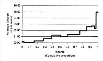
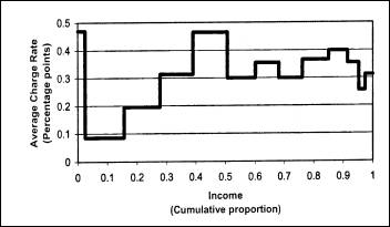
This method is based on the premise of testing the progressiveness and regressiveness of the potential effects of the implementation of a policy (or policies). The effects of a policy change are considered progressive if the financial burdens/gains increase/decrease with the income level. On the other hand the effects of a policy change are regressive if the financial burdens/gains decrease/increase with the income level. The notion of progressivity/regressivity is linked to the household’s ability to pay the increased liability due to the policy change. It can best be explained with the example of taxes imposed by government. A tax regime can be considered progressive if the average tax rate (total tax paid as a proportion of income) increases with income, i.e. average tax burden is higher for a richer household than of a poorer household. Similarly a tax regime is defined as regressive if the average rate falls with income. An income tax regime with tax-free allowances and with marginal tax rates that increases with income is an example of a progressive tax scheme. On the other hand a Value Added Tax is an example of a regressive tax given that it is independent of the ability to pay. Crawford (2000) used the progressivity/regressivity method in examining the distributional effects of the London congestion charging scheme (see Box 5).

STEPS INVOLVED

The progressive/regressive method involves the following steps:

Step 1: Establish the extent of the effects of the policy change. For example, if the change in policy involves an increase in a particular class of rail fare and for a particular route then establish the number of trips that will be affected by the fare increase. This can be established using survey data from other studies or through the commissioning of a study for this purpose;

Step 2: Identify and re-arrange the effects on the basis of the variable of interest (e.g. income levels) and calculate the financial implications of the policy changes on different groups. For example, in the case of the rail fare increase, calculate the total effects of the fare increase on each income group; and

Step 3: Calculate the average group effects as a proportion of income over a period and test the progressivity/regressivity of the policy change. This can be done with visual inspections by plotting average group effects against cumulative income percentiles or by making use of econometric techniques.

Box 5: Distributional effects of the London Congestion Charging Scheme

Crawford (2000) provides the details of the study. The following summarises the methodology and findings of the study:

(i) The London Area Transport Study (LATS) data, provided the number of trips made by members of households using different modes of transport affected by congestion charging. The LATS also provided information about origins and destinations, journey purposes, trip length, frequencies, gender, ethnic origin and banded household income;

(ii) Average incomes of household within each band were calculated from a family expenditure survey. These figures have helped in the calculation of the average weekly charges for different income percentiles;

(iii) The plots of the average weekly charges against the cumulative income percentiles (Figure 1) and the average weekly charges as a proportion of income against the cumulative income percentiles (Figure 2) were used to verify the progressiveness/regressiveness of the London congestion charging scheme.

(iv) On average the households towards the top of the distribution face higher liabilities than the households towards the bottom ((Figure 1);

(v) Apart from the households at the bottom of the distribution, the scheme can be considered progressive up to about the middle of the income distribution (Figure 2), i.e. average charge increases with ability to pay as we move from poorer households to the households at the middle of the income distribution. However, the scheme cannot be considered progressive from the middle to the high end of the income distribution.

Figure 1: Average weekly charges and income

FIGURE 2: AVERAGE CHARGE RATE AND INCOME

B Key points

· The progressivity/regressivity method is suitable for analysis of the effects of a policy change on different social groups. The main tenet of the method is based on the analysis of the potential financial effects of the policy change on different social groups;

· Such analysis may make use of suitable data from other studies (for example, transport study data in the area concerned). In the case of non-availability of such data a study with limited scope may need to be commissioned; and

· Establishment of the incomes of the households within different income bands is one of the crucial factors in this type of study.

G Remember

· It is important to remember that a household (or households) within an income band may face charge rates that are substantially different from those of another household (or other households) within the same income band. This is due to the use of average effects on the households under this income band;

· The analysis is based on the existing travel patterns. It does not take into account the potential effects of the new policy (policies) on travel behaviour.

ü Extension of the method

· The concept may further be extended to capture the effects of the policy change on gender, ethnic groups, spatial subdivisions etc.

Method for Rapid Assessment of the Gains by the Poor in a Workfare Programme

Ravallion (1999) has proposed the method to be used for rapid assessment of the likely gains to the poor from a workfare program – a programme that requires the participants to do physical work to obtain benefits. These programmes are common during a crisis such as macroeconomic or agroclimatic shocks when the employment opportunities for the poor are negligible. Workfare programmes provide short-term low-wage employment for able bodied persons in the crisis striken areas. An example of such a programme is the food for work programmes in different developing countries that employ labourers for improvement and maintenance of infrastructure, like roads, by paying wages in food. In these situations it is difficult to conduct detailed analysis and the data are far from ideal. The method addresses two main questions: (i) how much impact on poverty can be expected from the programme? (ii) is there any opportunity to modify the programme to enhance the impact on poverty?

The benefit gain to the poor as a proportion of the total public spending is given by:

and

Where:

· B is the total gain to the poor and B = NW+IB, where NW is the wages net of foregone income from other work or other costs of participation and IB is the indirect benefits to the poor when created assets become the public goods in poor neighbourhoods;

· G is the total government spending for the programme;

· is the budget leverage, C is the private co-financing from non-poor;

· is the labour intensity, W is the wage received by the poor labourers and L is the leakage to the non-poor;

· is the targeted labour earnings;

· is the net wage gain;

· is the targeted indirect benefits, SB is the total assets created to the whole population;

· is the benefit-cost ratio of the intervention; and

· is the share of net wage gains in total cost.

3Additional notes

NW/W is probably the most difficult variable to estimate in the analysis of a workfare programme. Its value will be 1 if the labourers for a workfare scheme were previously unemployed and there are no other participation costs incurred by the poor. But this is an unrealistic proposition as poor people cannot afford to be unemployed. If the probability of a labourer finding a job without the workfare programme is P^* at a wage rate of W^*, while P is the probability of finding some sort of job for the same worker with the workfare programme – the value of P may not be same as P^* due to the change in working opportunities with the introduction of the workfare programme. Now with the workfare wage rate of W the expected income gain of the particular worker will be PW^* + (1-P)W. The expected net wage gain (NW) to the particular worker will be PW^* + (1-P)W - P^*W^* that can be re-arranged as (1-P)W-(P*-P)W^*. In the case when P=P^* (i.e. the introduction of a workfare programme does not have any effect on the probability of finding a job for a worker) then the value of NW will be (1-P)W. When there is no possibility of finding a non-workfare job by the poor with and without the programme then P=P^*=0, i.e. NW = W and NW/W = 1. However, this is a very unlikely situation. Therefore, generally the value of NW/W will be lower than 1.

G Remember

· The method requires several assumptions. The success of the method depends on the accuracy of these assumptions.

· It is preferable to conduct sensitivity analyses with the key parameters in order to draw valid conclusions.

Box 6: EXAMPLE OF THE RAPID APPRAISAL OF THE WORKFARE PROGRAMME

Let us assume that two workfare programmes are introduced in two countries – while one in a middle-income country (MINC) that is experiencing high unemployment due to microeconomic stabilisation and reform programme, the other in a low-income country (LINC) hit by severe floods. The following table (Table 4) shows the calculations of the different variables mentioned above along with the assumptions made

Table 4: cost-effectiveness of the workfare programmes for a middle-income country (MINC) and a low-income country (LINC)

Variable	Variable Values		Assumptions & explanations
	MINC	LINC
G + C G	1	1	For MINC and LINC the private co-financing (C) is assumed negligible. Therefore, the budget leverage in both the cases is assumed to be 1.0.
W + L G + C	0.33	0.5	It is assumed that the program in the MINC will be less labour intensive than the LINC. Therefore, it is assumed that the labour wages will comprise 33% for the MINC and 50% for the LINC, i.e. (W+L)/(G+C) values will be 0.33 and 0.5 for MINC and LINC respectively.
W . W + L	1	0.75	The aim of the workfare programme is to provide work for as many people as possible without undermining the incentive to take regular jobs when they are available. This is why generally the workfare wage is often very low. Under such circumstances in the case of MINC the employment opportunities are unlikely to attract people who are not poor. Therefore, the leakage to the non-poor will be negligible in the case of MINC. On the other hand in the case of LINC often the wage rate is tied to the statutory wage rate for the agriculture labour that is often above the wage rate for casual agricultural labour. This high wage rate will attract workers who are non-poor or unemployed. Also it is often observed that the people who manage the program do not often favour the poorest. Therefore, a leakage of 25% of the total wages to the non-poor is assumed. The value of targeted labour earnings (W/W+L) is calculated at 0.75.
NW W	0.6	0.75	In the case of MINC is it is assumed that the probability of finding a job for an average programme participant of the workfare programme is 0.4 and there will be no change in the probability with the introduction of the programme. Then the value of NW will be 0.6W. Hence the value of NW/W will be 0.6. In the case of LINC the net wage gain is assumed as 0.75, higher than the MINC. Please see an additional note below explaining different aspects of this parameter.
IB SB	0.2	0.25	In the MINC as the programme does not attempt to target poor areas, the poor are as likely to benefit as the non-poor indirectly from the programme. Therefore, the value of IB/SB is assumed as 0.2, the existing poverty rate of the MINC. However, in the case of LINC the value of IB/SB is assumed at 0.25 – slightly higher value than the MINC. This assumption is based on the premise that the benefits to the poor will be higher due to the secondary effects of the programme – like the second-round employment effects due to higher farm productivity.
SB . G + C	1.0	0.5	It is assumed that in the case of MINC the generated benefits are sufficient to cover the costs. However, in the case of LINC it is assumed that due to the high labour intensity of the programme the benefits only cover a half of the costs.
B (current & future G gains to the poor)	0.40	0.41	For LINC: NW/G+C =0.75*0.75*0.5 = 0.28; IB/NW = 0.25*0.5/0.28 = 0.44; B/G = 1*0.5*0.75*0.75*(1+0.44) = 0.41
Cost of 1$ overall gain to the poor	2.50	2.50	The cost of transferring $1 amount of overall benefits to the poor will cost $2.5 for both MINC and LINC.
Current earning gain by the poor per $1 investment – CB/G	0.2	0.28	CB considers the current benefits only, i.e. IB=0.
Cost of $1 current gain to the poor	5.00	3.60	The cost of transferring $1 amount of immediate benefits to the poor will cost $5.00 in the MINC and $3.66 in the LINC.

4 Summary

Poverty reduction is one of the overarching objectives of the World Bank. Projects, particularly those with explicit poverty reduction objectives, should therefore be assessed for their contributions towards poverty reduction. At a minimum this should include a distributional analysis such as a Transport Economic Efficiency (TEE) table, whereby the groups that gain and lose are clearly identified.

A weakness of the traditional transport cost benefit analysis is that it does not inform us who the final beneficiaries of the project will be. There is no reason to suppose that travellers’ benefits are a good proxy for the incomes of those affected in the final markets. Whilst techniques are available that trace the manner that transport benefits feed into final markets, such techniques are not well developed and consequently will be beyond the resources of most appraisals. Most appraisals will therefore require distributional analysis to be based on the incidence of benefits accruing to travellers and vehicle operators (i.e. a TEE distributional analysis). Whilst not exact such an assessment will at the very least be indicative.

If possible some attempts should also be made to supplement the TEE analysis with an estimate of the ultimate beneficiaries of the project. There are several methods by which this can be done. The choice of a method depends on the type of project being appraised and the size of that project. A method involving detailed modelling and calculation of poverty impact indicators suitable for the appraisal of a multi-million dollar urban metro scheme will be wholly unwarranted for a small rural road project where simple market analysis will probably be sufficient.

Availability of data and resources are also key factors that will influence the choice of method. The quality of the analysis depends on the quality of the available data. The cost of obtaining and manipulating data often form a significant element of the cost of an appraisal. In many instances rational assumptions will also have to be made in the absence of sufficient data. Testing the sensitivity of the poverty analysis to these assumptions will help in making an informed decision.

A further issue that has to be considered is the issue of project selection. Without doubt some projects will be more beneficial for the poor than other projects, and some projects will have higher Internal Rates of Return (IRRs) than other projects. The difficulties arise when projects with the highest IRRs have the lowest poverty impacts and vice versa. Is the decision taker to trade off the economic rate of return against the poverty impact (i.e. some form of poverty -weighted rate of return approach)? Or is a sequential approach taken in which, within the set of projects that satisfy the economic efficiency test, those that are most pro-poor are selected? This is a policy matter and the answer may not be the same in each country. In the absence of a country specific decision process this Note has suggested an approach that could be used. Such an approach uses cost effectiveness analysis as a screening tool and economic efficiency analysis for final project selection.

5 Glossary of terms:

Conversion Factor (CF): Ratio between the economic price value and financial price value for a project input and output that can be used to convert the constant price financial values of project benefits and costs to economic values and vice versa.

Discount Rate: A percentage rate at which the value of equivalent benefits and costs decrease in the future compared to the present. The discount rate is used to determine the present value of future costs and benefits.

Financial Net Present Value (FNPV)/ Economic Net Present Value (ENPV): The difference between the financial/economic present value of the benefit stream and the financial/economic net present value of the cost stream for a project. The present value is calculated using a discount rate usually 12%

Poverty Impact Ratio (PIR): The proportion of the total benefits of a project (NPV) that accrues to the poor.

Present Value (PV): The value at present of an amount to be received or paid at some time in the future – determined by multiplying the future amount by a discount factor.

Standard Conversion Factor (SCF): The ratio of economic price value of all goods in an economy at their border price equivalent values to their domestic market price value. The SCF is generally less than one. For economic analysis using world price numeraire, it is applied to all project items valued at their domestic market price values for conversion to their border equivalent value. There is no need of such adjustments for the items valued at border price equivalent.

6 FURTHER READING:

Asian Development Bank (1994) Handbook for Incorporation of Social Dimensions in Projects, Asian Development Bank, Manila.

Asian Development Bank (1997) Guidelines for the Economic Analysis of Projects, Asian Development Bank, Manila.

Asian Development Bank (2001a) Handbook for Integrating Poverty Impact Assessment in the Economic Analysis of Projects, Economics and Development Resource Centre (EDRC), Manila.

Asian Development Bank (2001b) Report and Recommendation of the President to the Board of Directors on a Proposed Loan to the People’s Republic of China for the Guangxi Roads Development Project, Asian Development Bank, Manila.

Baker J L (1999) Evaluating the Poverty Impact of Projects: A Handbook for Practitioners, World Bank, Washington D.C.[Also available online at http://wbln0018.worldbank.org/HDNet/HDdocs.nsf/socialfunds/3cc655b089989b7d852568a30074c041/$FILE/Evaluating%20Poverty%20JudyBaker.pdf]

Barone , M. and Robelo, J. (2003) Potential Impact of Metro’s Line 4 on Poverty in the Sao Paulo Metropolitan Region (SPMR). World Bank, Washington DC, USA. [Also available online at http://www.worldbank.org/transport/urbtrans/poverty_14_sp.pdf]

Crawford I A (2000) The Distributional Effects of the Proposed London Congestion Charging Schemes (Briefing Note No. 11), The Institute for Fiscal Studies, London

Fujimura M and Weiss J (2000) Integration of Poverty Impact in Project Economic Analysis: Issues in Theory and Practice (EDRC Methodology Series Number 2), Asian Development Bank, Manila.

Gannon, C. and Liu, Z. (1997) Poverty and Transport (Discussion Paper No. TWU-30), World Bank, Washington D.C.

[Also available online at http://www.worldbank.org/transport/publicat/twu-30.pdf]

Gajewski G R and Luppino M, (2003) Poverty Reduction and Road Project : A Perspective Estimation Method (Working Paper of Asian Development Bank and Louis Berger Group), Asian Development Bank, Manila (Also available online at http://www.ecomod.net/conferences/ecomod2003/ecomod2003_papers/Gajewski.pdf)

Gwilliam K (2000) “Transport Project Appraisal at the World Bank”, paper presented to TRANSTALK seminar on appraisal methods for transport projects. Brussels, June 2000.

[Also available online at http://www.worldbank.org/transport/pol_econ/ea_docs/brussels.pdf]

Hajj H and Pendakur V S, (2000) Roads Improvement for Poverty Alleviation in China (Working Paper No. 1), World Bank, Washington D.C.

Hansen S (2000) Framework in Measuring Poverty Impact of Transport Projects (Final Report), Bekkestua, n.p.

I T Transport (2002) Feasibility and Formulation Report Uganda: Road Sector Programme Support - Phase 2 (District Roads Component, National Gravel Roads Component, National Labour Based Training Component), Danida, Copenhagen

Khandker S R and Chowdhury O H (1996) Targeted Credit Programs and Rural Poverty in Bangladesh, The World Bank, Washington D. C.

Powers T (1989) “A Practical Application: The IDB Experience” The Impact of Development Project on Poverty, OECD, n.p.

Ravallion M (1998) Poverty Lines in Theory and Practice, The World Bank, Washington D. C.

Ravallion M (1999) “Appraising Workfare”, The World Bank Research Observer, Vol. 14, no. 1 (February 1999), pp. 31-48.

Ravallion M (2000) The Mystery of the Vanishing Benefits: An Introduction to Impact Evaluation, World Bank, Washington D. C. [Also available online at www.worldbank.org/html/dec/Publications/Workpapers/wps2000series/wps2153/wps2153.pdf]

Squire L & Van der Tak H G (1975), Economic Analysis of Projects, Johns Hopkins University Press, London.

Srinivasan T N (2001) Growth and Poverty Alleviation: Lessons from Development Experience (ADB Institute Working Paper 17), Asian Development Bank Institute, Tokyo.

Van de Walle D and Cratty D (2002) Impact Evaluation of a Rural Road Rehabilitation Project, World Bank, Washington D. C. [Also available online at http://poverty.worldbank.org/files/11258_Dwalle-Impact-Rural_Roads.pdf ]

Van de Walle D (2002) “Choosing Rural Road Investments to Help Reduce Poverty”, World Development, Vol. 30 No. 4, pp 575-589.

Wood W G (2002) “Private Public Partnerships in Toll Roads in PRC”, A paper prepared for the ADB/PPIAF Conference on Infrastructure Development – Private Solutions for the Poor: The Asian Perspective held from 28-30 in Manila, Philippines.

World Bank (1994), OP 10.04: Economic Evaluation of Investment Operations, Operational Manual Volume II Analysis, World Bank, Washington DC, USA.

[Also available online at

http://wbln0018.worldbank.org/Institutional/Manuals/OpManual.nsf]

World Bank (1998) Handbook on Economic Analysis of Investment Operations, World Bank, Washington D.C. [Also available online at http://www.worldbank.org/education/economicsed/project/projwork/Handbook.pdf]

World Bank (2001) World Development Report, 2000/2001: Attacking Poverty, Oxford University Press, New York.

ANNEX I

APPROXIMATION OF INCOME SHARE OF THE POOR

ANNEX I

Approximation of Income Share of the Poor

ADB (2001a) provides the following formula for calculation of income share of the poor with an example from Vietnam.

Y_p = ((1-PG)*PL*POP*HC)/(GDP_pc*POP)

= ((1-PG)*PL*HC)/GDP_pc

Where Y_p = income share of the poor.

PL = poverty line annual income per capita.

PG = poverty gap index which is defined as the mean distance below the poverty line as a proportion of the line. The mean is formed over the entire population with non-poor having a zero poverty gap. Ravallion (1998) and Khandker and Chowdhury (1996) provide details of the theories and practices concerning poverty lines.

HC = headcount poverty index (a ratio of number of people below the poverty line to the total population) which is given by:

HC=POP_p/POP where, POP_p is the population who live in households with per capita consumption below the poverty line.

POP = total population.

GDP_pc = GDP per capita.

An illustrated example of calculation of Y_p with 1998 data from Vietnam:

PL = 1,790,000 dong based on the 1998 Vietnam Living Standard Survey (VLSS). However, this figure is not directly comparable with the international lower poverty threshold of US$1 per day in Purchasing Power Parity (PPP) prices of 1985 since this is a nominal figure;

HC = 0.374 (i.e. 37.4% of the population live below poverty line);

PG = assumed as 0.095 (i.e average income shortfall of the poor below the poverty line is 9.5%);

GDP_pc= dong 4,790,558 in 1998 nominal price.

Y_p = (1-0.095)*1,790,000*0.374/4,790,558

= 0.126

ADB (2001a) also provides country-specific data on the income share of the poor for developing countries in Asia.

ANNEX II

CASE STUDY 1:

THE JAMUNA BRIDGE

ANNEX II

SALIENT FEATURES OF THE JAMUNA BRIDGE STUDY

Background

A river system, constituted by the Jamuna, the Meghna and the Padma rivers, physically divides Bangladesh into three different regions - East, Southeast, and Northeast. At the time of conducting the study, there were numerous problems (for example, siltation of the riverbeds, erosion etc.) of crossing the rivers using ferries and boats. The Project was intended to provide an all-weather crossing for the East-Northwest traffic with the provision of the following: (i) a 4.8 km-long and 18.5 m-wide bridge with four road lanes and sidewalks; (ii) two viaducts, about 128 m-high; (iii) two guide bunds, about 2.2 km each and a flood protection bund on the east bank; (iv) two approach roads, about 16 km to the east and 14 km to the west (two-lane single carriageway with paved shoulders); (v) measures to mitigate the project's environmental impact; (vi) implementation of a resettlement plan; and (vii) technical assistance for project management. The bridge site, 7 km south of Sirajganj district headquarters, was selected after extensive studies of 10 potential sites. The total project cost of $696 million was co-financed by ADB, Overseas Economic Cooperation Fund (Japan), IDA, and the Government of Bangladesh. The bridge was opened for traffic operations in 1998.

Financial and Economic Analysis

Important assumptions:

· The project life after the bridge opens to traffic: 50 years;

· A traffic growth of 5% per year from 1998-2025. It was assumed that there would be no increase in traffic after 2025 as bridge capacity would be fully exhausted by 2035. The analysis considered three types of traffic – light passenger vehicles, buses and trucks.

· The reduction in waiting time and vehicle operating costs would generate additional passenger and freight traffic on the bridge. The newly generated traffic was estimated based on the price elasticity of demand for transport services: -1.0 for light vehicles, -1.5 for buses, and -0.6 for trucks, respectively. The assumption was that the generated traffic would be build up gradually: 20 percent of the total volume in 1998 to 40 percent, 50 percent, 60 percent, 70 percent, 80 percent, 90 percent, and finally 100 percent in 2005;

· While the financial revenue for the bridge comprised toll revenues from diverted and newly generated traffic and electricity interconnector fees, financial costs comprised the investment cost plus operating and maintenance costs of the bridge;

· Economic benefits of the project included: (i) VOC savings from diverted traffic; (ii) travel time savings from existing passenger and freight traffic; (iii) benefits from the generated traffic (equal to the gain in consumer surplus plus the financial toll revenue); (iv) the benefits of not constructing a stand-alone power inter-connector; (v) the cost savings by not improving the ferry system that existed at the time of the appraisal; (vi) the value of the increase in truck waiting time saved from year 2000 onwards by not operating the ferry system that existed at that time; (vii) the environmental benefits of preventing embankment erosion in areas close to the bridge and increase in agricultural production;

· The time saving values were not adjusted as labour was assumed to receive its market price (SWRF = 1). The appropriate conversion factors helped in the adjustments of the economic values of the investment cost items. The shadow exchange rate factor of 1.304 was used for converting the value of tradables to the domestic price numeraire.

TEE Distribution Analysis

· The benefits that were distributed comprised the following: In the Project's case, the difference between financial and economic flows derives from two factors: (i) difference between financial and economic flows of project inputs and outputs that have conversion factors different from unity (NPV_eco - NPV_fin) ; and (ii) the economic benefits that were not captured as financial benefits (NPV_eco);

· The study used a discount rate of 12.21 percent;

· The gains/losses were distributed among light vehicle passengers, bus passengers, truckers/shippers, power company, government, ferry operators and locality as a whole;

· While the vehicle owners, bus passengers, truckers/shippers, power company and locality were the gainers, the government/aid agencies and ferry operators were the losers from the Project;

Table A-1: Distribution Analysis: Bangladesh Jamuna Bridge Project (Million Taka, in 1974 price at 12.21% discount rate)

Items	FNPV	ENPV	ENPV-FNPV	Light Vehicle Passenger	Bus Passenger	Truckers/ Shippers	Power Company	Government	Locality	Ferry Operator
Cost Savings and Consumer Surplus
Light Vehicles	0.0	606.2	606.2	627.0				(20.8)
Buses	0.0	1,904.7	1,904.7		1,951.6			(46.9)
Trucks	0.0	27,181.1	27,181.1			27,936.8		(755.7)
Avoided truck waiting time	0.0	3,157.3	3,157.3			3,157.3
Toll revenue
Diverted traffic
Light Vehicles	74.7	0.0	(74.7)							(74.7)
Buses	588.3	0.0	(588.3)							(588.3)
Trucks	1,177.8	0.0	(1,177.8)							(1,177.8)
Generated Traffic
Light Vehicles	29.4	29.4	0.0	0.0
Buses	203.6	203.6	0.0		0.0
Trucks	627.4	627.4	0.0			0.0
Electricity Inter-connector fees	344.1	0.0	(344.1)				(344.1)
Savings on stand-alone power interconnector	0.0	2,888.3	2,888.3				2,888.3
Savings from avoided
Costs of ferry system
Ferry purchse	0.0	327.4	327.4					327.4
Dredging and maint.	0.0	460.1	460.1					460.1
Environmental benefit	0.0	456.9	456.9						456.9
Loan	19,851.2	0.0	(19,851.2)					(19,851.2)
Government grant	2,455.4	0.0	(2,455.4)					(2,455.4)
Total benefits	25,351.9	37,842.4	12,490.5	627.0	1,951.6	31,094.1	2,544.2	(22,342.5)	456.9	(1,840.8)

Items	FNPV	ENPV	ENPV-FNPV	Light Vehicle Passenger	Bus Passenger	Truckers/ Shippers	Power Company	Government	Locality	Ferry Operator
Investment costs
Main bridge	(8898.5)	(11178.7)	(2280.2)					(2280.2)
River training works	(9794.3	(12396.1)	(2601.8)					(2601.8)
Approach roads	(2056.9)	(2418.3)	(361.4)					(361.4)
Technical assistance	(901.2)	(1016.2)	(115)					(115)
Others	(2041.2)	(2041.2)	0					0
Operating & maintenance costs	(1017.2)	(1017.2)	0					0
Total Costs	(24709.3)	(30067.7)	(5358.4)	0	0	0	0	(5358.4)	0	0
Gains or Losses	642.6	7774.7	7132.1	627	1951.6	31094.1	2544.2	(27,058.3)	456.9	(1840.8)

Note: The calculated net loss to Government/Economy -27,058.3 (i.e -22,342.5-5358.4+642.6)

ANNEX III

CASE STUDY 2:

THE TAJIKISTAN ROADS PROJECT STUDY

ANNEX III

SALIENT FEATURES OF THE TAJIKISTAN ROADS PROJECT STUDY

Background

Among the Central Asian republics Tajikistan is the poorest. There was a decrease in economic activity and a dramatic increase of poverty in Tajikistan after the demise of the former Soviet Union. The rehabilitation of the country's road infrastructure necessary to sustain the economic recovery now is under way.

The project scope included the rehabilitation of approximately 80 km of the most deteriorated sections of the Dushanbe-Khulyab road and improvement of approximately 150 km of rural roads with appropriate drainage facilities. The total project cost was $26.8 million with ADB being the main contributor ($20 million). The project started in late 2000.

Economic Analysis

· The analysis period: 24 years (2001–2024), including about 4 years for project implementation. All benefits and costs were estimated in constant 2000 prices;

· With no revenues involved and no financial analysis carried out, the analysis used world price numeraire for calculation of economic values. In the backdrop of the uncertainty of currency exchange rates, the project cost estimation was done in US dollars.

· A standard conversion factor (SCF) of 0.9 was used to adjust the nontradable inputs and a shadow wage rate factor (SWRF) of 0.75 was used for valuation of unskilled labour;

· The Project's economic benefits primarily included: vehicle operating costs (VOCs) savings from normal traffic, passenger time savings, and benefits arising from generated traffic (VOC savings estimated as a half the value for normal traffic);

· The study used the highway design and maintenance model (HDM-Manager) for estimation of passenger and freight vehicles’ VOCs;

· VOC savings comprise the largest category of benefits – more than 85 percent of the total benefits. EIRRs were calculated for the national road sections and for the overall Project. The EIRR for the overall Project was 15.9 percent, whilst the EIRRs for the national road sections ranged from 14.2 to 25.4 percent. The study did not conduct any sensitivity test in the case of economic analysis.

Distribution Analysis

· The study calculated disaggregated road user benefits (VOC and time savings) for 4 classes of passengers vehicles and 3 classes of freight vehicles;

· The study conducted field surveys in the project area that involved passengers, drivers and farmers in order to assess the structure and performance of the transport market. The distribution analysis made use of these findings. Such surveys also captured the social groups of the users. They also helped to determine the proportion of operating cost savings that would be passed from vehicle owners to the users;

· The survey results found that the market for passenger transport services was fairly competitive. Small owneroperators dominated 80 percent of the market that made it substantially competitive. The analysis also showed that the drivers could not extract abnormal monopoly rents from owning and operating vehicles on project roads. Farmers were the big users of the road. They sold their produce themselves as the prices offered by the middlemen were not competitive enough. 80% of the farmers who sold their produce locally cited high transport costs as the main reason for doing so (on average about 20% of the output price). The study identified several barriers that made the transport and agriculture markets from being fully competitive;

· The study made a generous use of secondary information apart from primary information. The main secondary information source was the Tajikistan Living Standard Survey (TLSS) conducted in 1999 by the State Statistical Agency (SSA). Among other, the TLSS information helped in making valid conclusions on traffic growth elasticities;

· The proportion of users’ benefits that would eventually be passed to vehicle users was 20% for pickups and articulated trucks and 50% for cars and buses;

· The stakeholders among whom the net benefits were distributed were: (i) passenger users, (ii) freight users, (iii) vehicle owners, (iv) labour, and (v) Government/economy. Given the non-recovery of the costs associated with the construction and maintenance of the roads, these costs were apportioned to the government;

Poverty Impact Analysis

· Based on the survey results and the poverty line estimates of the TLSS the study assumed that 60 percent of drivers, farmers, and passengers using the transportation services in the project area were poor and the figure was used in the calculation of the passengers’ benefits accruing to the poor;

· The study assumed that 20% of the freight benefits and 30% of the vehicle owners’ net benefits would accrue to the poor;

· As the plan was to use unskilled labour in the rehabilitation of the project roads, the assumption was that the poor labourers would get 80% of the total labour benefits;

· The study initially assumed the poor income share proportion of 0.1. The calculated PIR was 0.62 under this assumption. However, the TLSS provided a headcount poverty incidence of over 80%. This practically means that project would not have any positive poverty reduction impact if the national and project area poverty incidence figures were similar. Sensitivity analysis revealed that the PIR could be as high as 0.8 under the assumption that 85% of the cost savings would be passed to passengers and freight transport users. The study showed the positive link between transport services market competition and the poverty reduction impact of project interventions.

Table A-2: Distribution of Net Benefits and Poverty Impact Ratio for a Tajikistan Road Rehabilitation Project (US$1,000 in present value at 12% discount rate)

	FNPV	ENPV	Difference (ENPV-FNPV)	Passenger Users	Freight Users	Vehicle Owners	Labour	Public Lender	Govt.
Inflow
Road users’ benefits	0	11,655	1,655	4,130	1,947	5,578
Loan	3797	0	(3797)					(3,797)
Outflow
Investment and O&M	(3797)	(3417)	380						380
Labour	(260)	(195)	65				65
Interest	(500)	0	500					500
Principal	(2000)	0	2000					2,000
Net Present Value	(2760)	8043	10,803	4,130	1,947	5,578	65	(1,297)	380	Total
Gains or Losses				4,130	1,947	5,578	65		(3,677)	8,043
Proportion of the poor (%)				60%	60%	30%	80%		10%
Net benefits for the poor				2,478	1,168	1,673	52		(368)	5,004
Poverty Impact Ratio				0.62

Note: The net loss to the public lender and government/economy is calculated at -3,677 (-2,760-1,297+380)

ANNEX IV

CASE STUDY 3:

THE RURAL ROAD POVERTY IMPACT STUDY IN UGANDA

ANNEX IV

SALIENT FEATURES of THE RURAL ROAD POVERTY IMPACT STUDY IN UGANDA

Uganda’s road network comprises about 9,500 km of national roads, 25,000 km of district roads, 2,800 km of urban roads and 30,000 km of community access roads. Of the national roads some 2,100 km are paved, the remainder being gravel surfaced and classified as A, B or C according to their importance. The majority of district and rural roads are gravel or earth, whilst community access roads range from well engineered roads to unimproved tracks.

The government’s 1996 10-year Road Sector Development Programme (RSDP) had a national roads focus, but the March 2002 update (RSDP 2) covering the period 2001-02 to 2010-11 is concerned with the entire road sector. Key provisions include, among other, increased use of labour-based methods for construction and maintenance, especially rural roads. This provision is made as the use of labour-based methods of road construction and maintenance offers considerable direct employment and poverty reduction benefits if compared to their equipment-based counterparts. A Government of Uganda’s White Paper published in 2002 relating to district, urban and community roads sets a target of the utilisation of labour based methods for 100% of the district road routine maintenance and 60% of periodic maintenance and rehabilitation by 2005-06.

The poverty impact analysis was conducted as a part of the district roads feasibility study in the northern part of Uganda for a potential road investment project with Danish government (Danida) assistance. The objective of the poverty impact analysis was to demonstrate to the policy makers the positive poverty impact of the adaptation of labour-based methods over its equipment-based counterparts. Findings of a 1999 cost comparison study between labour-based and equipment-based methods in Uganda facilitated the poverty impact analysis. The study results especially helped in making informed decisions concerning the proportions of different cost items (e.g. skilled labour, unskilled labour, materials, equipment etc.)

However, given the difficulty in assessing the proportion of income share of the poor and the proportion of users’ benefits from project investments accruing to the poor, the Poverty Impact Ratios (PIRs) were calculated for different proportions of income share of the poor and users’ benefits reaching the poor. This helped in making the case that the labour-based methods has higher poverty impact than equipment-based methods. The study used the World Bank’s RED model to calculate the road users’ benefits.

The other key assumptions of the study were the following:

· The unit cost of investment : US$4,500 per km for an average length of 25 km of road;

· The proportion of different cost items:

o Labour-based works: material 14%, labour 51%, equipment 23% and other cost 12%.

o Equipment-based works: material 8%, labour 6%, equipment 61% and other cost 25%.

· The ratio of skilled and unskilled labour:

o labour-based works: 10:90,

o equipment-based works: 50:50

· Shadow wage rate factor for skilled labour: 1.0

· Shadow wage rate factor for unskilled labour: 0.59 [†]

· Standard conversion factor: 0.89 [‡]

· Proportion of poor among unskilled labourers: 90%

Table A-3: Distribution of Net Benefits and Poverty Impact Ratio for a Rural Road Project in Northern Uganda (US$ in present value at 12% discount rate)

	FNPV	CF	ENPV	Difference (ENPV-FNPV)	Donor	Government	Skilled Labour	Unskilled Labour	Consumer
Benefits
Consumer Surplus		1	331,516	331,516					331,516
Donor's Grant	277,605		0	(277,605)	(277,605)
Government Grant
Costs
Material Costs	(21,946)	0.89	(19,532)	2,414		2,414
Skilled Labour	(7,324)	1	(7,324)	0			0
Unskilled Labour	(12,414)	0.59	(7,324)	5,090				5,090
Equipment	(167,338)	0.89	(148,931)	18,407		18,407
Other costs	(68,581)	0.89	(61,037)	7,544		7,544
Net Present Value	0		87,366	87,366	(277,605)	28,365	0	5,090	331,516

	Government	Skilled Labour	Unskilled Labour	Consumer	Total
Gain or Losses (NEB-NFB)	28,365	0	5,090	331,516	364,971
Financial Investment	(277,605)				(277,605)
Benefits	(249,239)	0	5,090	331,516	87,366
Proportion of poor	30%	0	50%	30%
Benefits to poor	(74,772)	0	2,545	99,455	27,228
Poverty Impact Ratio	0.3117

Proportion of Costs under different construction technology options

	Labour-based methods	Equipment-based methods
Material	14%	8%
Labour	51%	6%
Equipment	23%	61%
Other costs	12%	25%

---

[*] The note only deals with the ex-ante method of distribution and poverty impact analyses. Various literature has recently been published dealing with the ex-post evaluation of poverty impact of projects (Baker, 1999; van de Walle and Cratty, 2002). The note also does not deal with the targeting of investment in poor areas as has recently been practiced in China by the World Bank. Hajj and Pendakur (2000) provides the details of the China approach

[†] Calculated using similar methodology proposed by Squire & van der Tak (1975)

[‡] Calculated using Uganda Bureau of Statistics’ four year data (1997/98 to 2000/01) on total values of imports, exports, import duty and export duty.